Bootstrap your own latent - A new approach to self-supervised Learning

year: 2020
paper: bootstrap-your-own-latent-a-new-approach-to-self-supervised-learning
website: YK Youtube; understanding-self-supervised-and-contrastive-learning-with-bootstrap-your-own-latent-byol
code:
connections: self-supervised learning, representation learning, SimCLR

---

Self-supervised image representation learning without negative pairs.
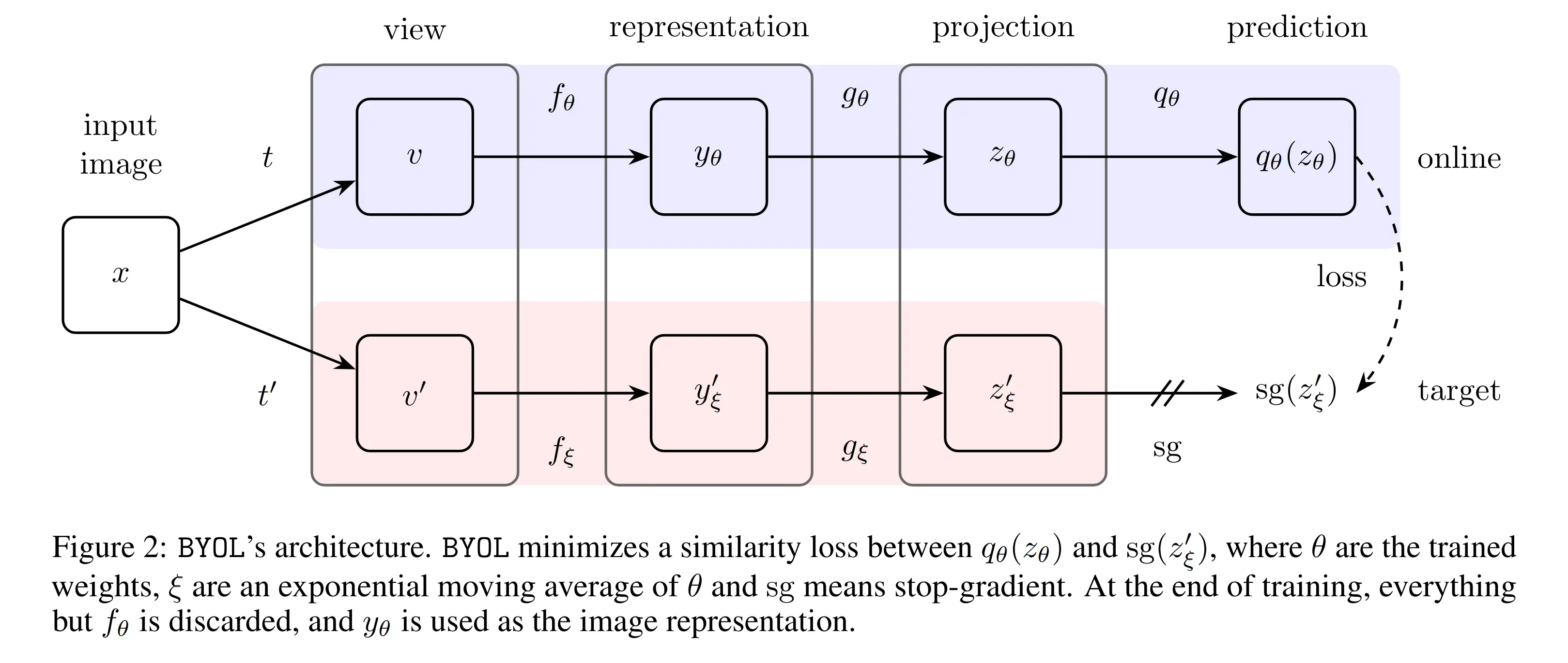
Two augmented views $v,v^{\prime }$ of the same image are fed through two networks. The online network ($\theta$) is encoder → projector → predictor. The target network ($\xi$) is encoder → projector only. The online network is trained to predict the target’s projection of the other view; the target’s parameters are a slow exponential moving average of the online’s, with stop-gradient on the target branch.

Slop below

Notation

$x$ … input image; $v=t(x),v^{\prime }=t^{\prime }(x)$ … two augmented views, with $t,t^{\prime }$ sampled from an augmentation distribution
$y_{\theta }=f_{\theta }(v)\in {\mathbb{R}}^{2048}$ … representation (the only thing kept after training)
$z_{\theta }=g_{\theta }(y_{\theta })\in {\mathbb{R}}^{256}$ … online projection
$z_{\xi }^{\prime }=g_{\xi }(f_{\xi }(v^{\prime }))\in {\mathbb{R}}^{256}$ … target projection (sg)
$q_{\theta }(z_{\theta })$ … predictor’s guess of $z_{\xi }^{\prime }$
$\overline{\cdot }$ … L2-normalised vector

Methodology

The training signal is “the online net should predict, from view $v$, what the target net produces from the other view $v^{\prime }$”. The loss measures how well that prediction lines up with the actual target projection:

$${\mathcal{L}}_{\theta ,\xi }=\Vert \overline{q_{\theta }(z_{\theta })}-\overline{z_{\xi }^{\prime }}{\Vert }_2^2$$

i.e. squared Euclidean distance between prediction and target, after both have been L2-normalised. Equivalently $2-2\cos (q_{\theta }(z_{\theta }),z_{\xi }^{\prime })$: zero when prediction and target point the same way, $4$ when opposite. So the loss only cares about the direction of the projection in feature space, not its magnitude. The L2-normalisation step is what enforces that: we strip the norms first, then measure distance, so two projections pointing the same way score zero loss regardless of how long they were before normalising.

Why ignore magnitudes? In a learned representation, the direction of a feature vector is what carries semantic content. Two projections pointing the same way mean the same thing about the input, whether one has norm 1 and the other norm 100. Letting the loss penalise magnitude differences would just have the network spend capacity matching scales for no gain.

The loss above is one-directional (online sees $v$, target sees $v^{\prime }$). BYOL symmetrises: it also pushes $v^{\prime }$ through the online branch and $v$ through the target, computes the same loss, and sums. Each view ends up acting as both the input and the prediction target over the course of training, which doubles the signal for free. Gradients only flow through $\theta$. The target branch carries a stop-gradient and is never directly optimised.

The target’s parameters are an exponential moving average of the online’s:

$$\xi \leftarrow \tau \xi +(1-\tau )\theta ,\tau \in [0,1]$$

with $\tau$ cosine-scheduled from $0.996$ at the start of training up to $1$ at the end. Why a moving target instead of just copying $\theta$ each step? You need the target to be two things at once: stable enough that the online net has a coherent signal to chase from one step to the next, and fresh enough that it keeps absorbing the online net’s improvements (otherwise you’re just predicting a fixed random initialisation, which only gets you to ~19% top-1). The EMA interpolates between those, and the schedule shifts the balance over time: early in training the online net is far from converged so we want the target to follow it relatively quickly (smaller $\tau$); late in training the online net’s representations are close to good and we want the target to stop moving so the online net can settle (larger $\tau$, eventually frozen).

The projector $g$ and the predictor $q$ have the same architecture: Linear(2048→4096) → BN → ReLU → Linear(4096→256). The final 256-dim output is not batch-normalised, unlike in SimCLR (this seemingly small detail turns out to matter; see the BN callout below). Augmentations are SimCLR’s set: random crop with resize, colour jitter, Gaussian blur, and solarisation.

The reason the architecture is asymmetric (predictor on the online branch only, stop-gradient on the target) is that without those two choices, the trivial fixed point $z_{\theta }=z_{\xi }^{\prime }=c$ for any constant $c$ would be a global minimum of the loss. Both networks could just learn to output the same constant vector for every input and the prediction error would be zero. The predictor breaks the symmetry of the loss surface, and the stop-gradient prevents the target from gradient-descending into the constant solution alongside the online net. The next callout argues why this is actually enough to make the constant solution an unstable equilibrium rather than just a non-trivial one.

Why doesn't it collapse? (paper's hypothesis)

$\xi$ is not updated by gradient descent on $\mathcal{L}$. So there’s no joint loss being minimised over $(\theta ,\xi )$, and no a priori reason the dynamics should converge to a minimum at all. Same shape as a GAN: alternating updates, no joint objective.

Assume the predictor is optimal, $q^{\ast }(z_{\theta })=\mathbb{E}[z_{\xi }^{\prime }\mid z_{\theta }]$. Then in expectation the online gradient becomes

$${\nabla }_{\theta }\mathbb{E}\left[\sum _i\mathrm{Var}(z_{\xi ,i}^{\prime }\mid z_{\theta })\right]$$

i.e., $\theta$ is pushed to make $z_{\theta }$ maximally informative about $z_{\xi }^{\prime }$. Conditioning on a constant gives the worst predictor ($\mathrm{Var}(z_{\xi }^{\prime }\mid c)\ge \mathrm{Var}(z_{\xi }^{\prime }\mid z_{\theta })$ for any $z_{\theta }$), so collapse is an unstable equilibrium under this dynamic.

The slow EMA’s role: keep the predictor near $q^{\ast }$ while $\theta$ moves. A hard copy ($\tau =0$) would break the optimal-predictor assumption, and empirically destroys training.

BatchNorm is doing implicit contrastive learning

From an imbue replication study: removing BN from the projector/predictor MLPs makes BYOL collapse to random performance. Replacing BN with LayerNorm (which doesn’t mix examples) also collapses. So it’s the cross-batch interaction in BN, not normalisation per se, that prevents collapse.

Mechanism: BN forces activations to have zero mean / unit variance across the mini-batch. A constant projection across the batch is exactly what BN subtracts away. Every sample is implicitly pushed away from the batch mean, which acts as a soft negative pulled from the rest of the batch. Contrast is happening, just routed through batch statistics rather than an explicit InfoNCE term.

Caveat the BYOL authors raised in response: with LARS + weight decay (instead of plain SGD), BYOL can still learn without BN, though much worse and brittle to hyperparameters. Those tricks prevent collapse through different mechanisms (weight regularisation keeps the network from sliding into a degenerate constant solution). So BN isn’t the only anti-collapse mechanism, but it’s the most robust one in practice.

Robustness vs. SimCLR

No negatives → no dependence on a huge batch. BYOL is stable from batch 256 to 4096; SimCLR drops sharply below 4096.
Removing colour distortion: SimCLR loses 27 points (it was solving the contrastive task via colour histograms alone), BYOL only 13. BYOL has to predict the target’s full projection, not just discriminate, so it can’t shortcut to a single statistic.
EMA decay $\tau$ between 0.9 and 0.999 all work. $\tau =0$ (instant copy) destroys training. $\tau =1$ (frozen random target) plateaus around 18.8% top-1; still well above the 1.4% an untrained encoder gets, so even predicting a fixed random target is a non-trivial pretext task.