Encoding innate ability through a genomic bottleneck

year: 2024/08
paper: https://www.pnas.org/doi/pdf/10.1073/pnas.2409160121
website: From the connectome to AI and back by anthony zador (YT)
code:
connections: genomic bottleneck, regularization, compression, neural compression, transfer learning, indirect encoding

---

The genomic bottleneck is an approach to neural architecture design inspired by biology.

A “genomic” network (G-network) with far fewer parameters than a “phenotype” network (P-network) generates the initial weights of the P-network through a lossy compression scheme. This mimics how a small genome encodes the development of a complex brain, and creates networks with strong innate (zero-shot) capabilities and better transfer learning properties.

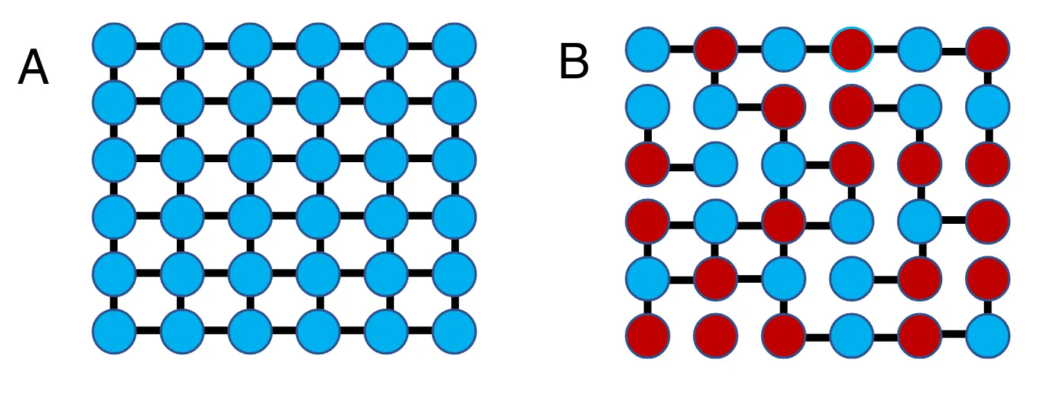
Simple rules can specify networks.

(A) A very simple nearest-neighbor wiring rule.
(B) A somewhat more complex rule (“only connect to nearest neighbors of opposite color”) leads to a more complex network.

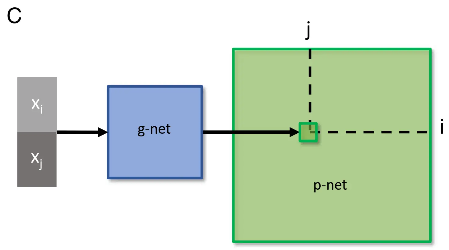
Network specification through a genomic bottleneck.

(C) The input to the genomic network (“g-network”) is a pair of neurons (pre- and postsynaptic) specified by binary strings. Each neuron has a unique label, consisting of a unique binary string. The two binary labels are passed through the g-network, which assigns the strength of the connection between the two neurons in the “p-network.” Because the number of parameters in the g-network is smaller than the number of parameters in the p-network, the g-network is effectively compressing the p-network.

G-Network Architecture & Function

The G-network is a small, typically feed-forward MLP, designed to act as a generative function, outputting the weights for the much larger P-network.

Its input consists of identifiers for a pair of neurons in the P-network: one pre-synaptic ($i$) and one post-synaptic ($j$). Each neuron across the entire P-network is assigned a unique binary label. They use gray code to encode the ids (TODO why? does it make the landscape smoother?).
To predict the weight $w_{ij}$, the G-network receives the 10-bit label for neuron $i$ concatenated with the 10-bit label for neuron $j$, forming a 20-bit input vector.

The paper’s MNIST example has a structure like 20 (input) → 30 → 10 → 1 (output). This tiny network, with only about 2,000 parameters, is responsible for generating the weights of the P-network, which has around 600,000 parameters.

The output of the G-network is a single scalar value, ${\hat{w}}_{ij}$, which is the G-network’s prediction for the connection strength (weight) between neuron $i$ and neuron $j$ in the P-network.

Each layer (or distinct weight matrix, like convolutional kernels or fully connected layers) is compressed by a separate G-network, which allows each G-network to learn the appropriate generative rules for different types of connections (e.g., convolutional vs. dense)(, and levels of abstraction?).

What is the G-network trained on?

The G-network is not trained directly on the primary task data (like images or rewards).
It’s trained on a supervised regression task: predicting the weights of the trained P-network.
After the P-network (e.g., a CNN for CIFAR-10) undergoes some training on its target task and its weights $W^{(n)}$ are updated, these weights become the training targets for the G-network. The G-net learns to map neuron identifier pairs $\{b_i,b_j\}$ to the corresponding P-network weight $w_{ij}^{(n)}$, typically by minimizing Mean Squared Error (MSE) between its prediction ${\hat{w}}_{ij}$ and the target $w_{ij}^{(n)}$.

Iterative Training ("Intermittent Training" / Co-optimization)

The G and P networks are trained in nested loops, simulating a co-evolutionary process where the “genome” (G-net) encodes developmental rules for the “phenotype” (P-net), which then learns through experience. When multiple G-networks are used (e.g., one per P-network layer), this process applies independently to each G-network/P-network component pair.

1. Inner Loop (P-net Learning): Train the P-network on its target task (e.g., image classification, RL) for a short period (e.g., a fraction of an epoch). Let the updated weights be $W^{(n)}$.
2. Outer Loop (G-net Learning): Freeze the P-network weights $W^{(n)}$. Train the G-network for several epochs to minimize the reconstruction error: $MSE({\hat{W}}^{(n)},W^{(n)})$, where ${\hat{W}}^{(n)}$ are the weights predicted by the current G-network using neuron IDs as input.
3. Initialization for Next Iteration: Use the G-network’s output ${\hat{W}}^{(n)}$ to initialize the P-network for the next round of inner-loop training ($W^{(n+1)}\leftarrow {\hat{W}}^{(n)}$).

Stability during early training ${\hat{W}}^{(n)}$ might be blended with the previous P-network weights or a random initialization using an annealing coefficient $ϵ(n)$: $W_n=ϵ(n)W_{n-1}+{\tilde{W}}_{n-1}(G)[1-ϵ(n)]$. This prevents the G-net from drastically disrupting the P-net early on.

To stabilize training when the G-network is still naive, its predictions

4. Repeat: This cycle is repeated for many “generations” (e.g., ~500 in the paper’s examples).

Size Relationship: G-Net vs. P-Net

The G-network is orders of magnitude smaller than the P-network layer it generates. This massive difference in parameter count is the genomic bottleneck.

• MNIST Example: P-network ≈ 6 × 10⁵ weights; GN30 (G-net with 30 hidden units) ≈ 2 × 10³ parameters → ~322x compression.
• CIFAR-10 Example: P-network layers up to 1.4 × 10⁶ weights; GN50 ≈ 1.5 × 10⁴ parameters → ~92x compression per layer.

This forces the G-network to learn compact, general rules for generating weights, rather than memorizing individual connections.

Compression as Regularization and Feature Extraction

By forcing the entire P-network weight specification through the tiny G-network, the process acts as a strong regularizer. It biases the system towards finding simpler connectivity patterns that are sufficient for the task.
Innate Ability: This results in P-networks that exhibit high performance at initialization (zero-shot), mimicking innate capabilities in animals.
Transfer Learning: The compressed representation often captures more fundamental, generalizable features of the task or data distribution. This was shown to enhance transfer learning, especially for lower layers in the CIFAR-10 → SVHN experiment, where G-network mediated transfer sometimes outperformed direct weight transfer. This parallels observations in biology where early sensory processing seems more conserved across species than higher-level processing.
Avoiding Overfitting/Shortcuts: The regularization effect can also lead to more robust solutions, potentially avoiding “reward hacking” issues seen in RL tasks like HalfCheetah when trained from random initialization.

Experiment Details

Supervised Learning (MNIST & CIFAR-10):

• High Compression & Innate Performance: Standard ANNs (MLPs for MNIST, CNNs for CIFAR-10) could be compressed by 100-1000 fold via the G-network while retaining high initial (“innate”) performance (e.g., 94% on MNIST with 322x compression, 76% on CIFAR-10 with 92x compression), often close to the fully trained P-network’s performance.
• Learning Dynamics: Compression provided a significant “hot start” (high initial accuracy) but didn’t necessarily accelerate the rate of subsequent learning on the same task compared to training from scratch (Fig 3E).
• Transfer Learning (Mixed Results):
  • MNIST → Fashion-MNIST: Transfer failed; initializing with MNIST-trained G-net weights hindered F-MNIST learning. This suggests overfitting on the simpler MNIST task/network.
  • CIFAR-10 → SVHN: Transfer was successful. G-network mediated transfer performed comparably to standard full-weight transfer, despite using ~92x fewer parameters. Transferring only lower layers via G-net sometimes outperformed direct transfer, suggesting the bottleneck effectively extracts generalizable low-level features. Transferring higher layers hindered performance, indicating dataset-specific features.
  • Feature Representation (MDS Analysis): Multidimensional scaling suggested the compressed MNIST network learned simpler, potentially more general features (resembling Gabors) compared to the uncompressed network (Fig 2E-G).
  Reinforcement Learning (Atari & MuJoCo):
  • High Compressibility in RL: Policies for Atari games (BeamRider, SpaceInvaders) using Dueling DQN architectures were also highly compressible (up to ~3500x) with minimal loss in initial performance.
  • Regularization Effect (HalfCheetah): For the continuous control task HalfCheetah (MuJoCo), G-network initialization not only achieved good compression and initial performance but also acted as a strong regularizer. P-networks initialized via the genomic bottleneck learned conventional gaits, avoiding the “reward hacking” behaviors (like flipping or tumbling) often seen when training from random initializations. This strongly suggests the compression forces the system towards simpler, more robust solutions.