kernel density estimation

Kernel Density Estimation

KDE is a way to estimate probability density functions from data samples without assuming any specific distribution shape. Given observations $x_1,x_2,\dots ,x_n$:

\hat{f}(x) = \frac{1}{nh} \sum_{i=1}^{n} K\left(\frac{x - x_i}{h}\right) $$ where $K$ is the kernel function (a smooth bump shape) and $h$ is the bandwidth parameter. Instead of dividing data into bins, KDE places a small smooth curve at each data point. These curves overlap and add up to create a [[continuous]] density estimate. The final result shows where data is concentrated without the arbitrary jumps you get from [[histogram]] bins. ![[kernel density estimate-1749804132743.webp|887x444]]

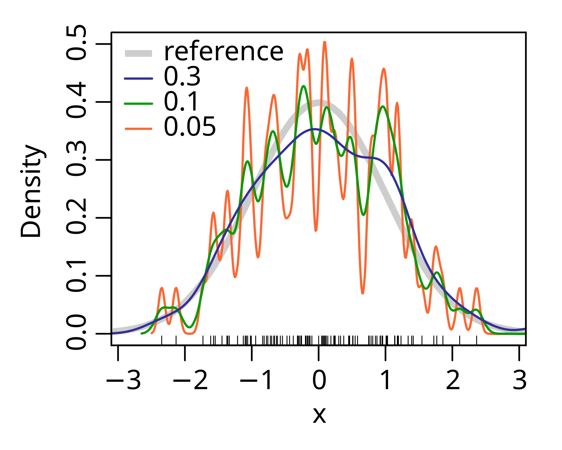
Bandwidth = sharpness

Small $h$ gives a sharp image where you see every detail (including noise). Large $h$ blurs everything together into smooth shapes. You need to find the sweet spot where real patterns are visible but noise is smoothed out.

Why KDE

KDE lets you visualize and analyze data distributions without forcing them into parametric forms. It reveals multiple modes, skewness, and other features that summary statistics miss. The tradeoff is that you need to choose the bandwidth carefully to balance detail against smoothness.

Why divide by $h$ outside the sum?

When we scale the kernel argument by $\frac{x-x_i}{h}$, we’re stretching the kernel horizontally by factor $h$. This makes each bump wider, but also increases its area by factor $h$. To maintain a proper probability density (integrating to 1), we must compensate by dividing by $h$. Without this correction, wider kernels would contribute more total probability mass, violating the requirement that $\int \hat{f}(x)dx=1$.

Gaussian kernel

The most common choice is the Gaussian kernel $K(u)=\frac{1}{\sqrt{2\pi }}{e}^{-\frac{1}{2}{u}^2}$, which places a normal distribution centered at each data point.

curse of dimensionality

KDE works great in 1-3 dimensions but struggles in high dimensions. The number of samples needed grows exponentially with dimension to maintain the same estimation quality.