TTS

Developmental Encodings Promote the Emergence of Hierarchical Modularity

Jessica Lowell${}^1$ and Jordan Pollack${}^1$

${}^1$DEMO Lab, Departmentl of Computer Science, Brandeis University, Waltham, MA 02453
jessiehl@cs.brandeis.edu

Downloaded from http://direct.mit.edu/isal/proceedings-pdf/alif2016/28/344/2326003/978-0-262-33936-0-ch058.pdf by guest on 14 April 2026

Abstract

While it has been observed (Hornby et al., 2001)by Hornby and colleagues in 2001 that developmental encodings in evolved systems may promote modularity, there has been little quantitative study of this phenomenon. There has also been little study of the factors driving the emergence of hierarchical modularity - modularity on multiple levels, in which the modules found at a finer-grained level can serve as elements in a coarser-grained network that is also modular - despite the fact that most fields with an interest in modularity, including biology and engineering, define hierarchy as an important aspect of modularity. We examine the effect of developmental encodings on the emergence of multiple levels of modularity through the lens of two developmental systems, GRNEAT and GENRE, and find evidence that developmental encodings promote this emergence of modular hierarchy.

Introduction

Below, we examine interactions between development and hierarchical modularity in artificial systems. Modularity, the organization of a system into a hierarchical system of interacting subparts, is observed in many systems both natural and engineered (Koza, 1992; Simon, 1996; Hartwell et al., 1999), and has become important as evolutionary systems are used in increasingly complex applications. Simulations of development, the process by which a mature phenotype is constructed from an organism’s genetic code, have been used in computational studies both in conjunction with and distinct from simulations of evolution. We briefly discuss modularity in evolution, followed by an overview of artificial development.

Modularity

Biological systems, including biological networks such as neural networks and bacterial metabolic networks, and other kinds of biological systems such as tissues (which are assembled from cells), tend to be modular. The definition of modularity is somewhat vague - though generally referring to the degree to which a system is composed of separable, recombinable components - and can be used differently in different fields and subfields. Bolker (2000)In 2000, Bolker attempted to define a list of characteristics of modularity that would be appropriate across different subfields and levels of study in biology, including greater internal integration of modules as compared to external integration, the ability to delineate modules from their surroundings, and module performance that is greater than the sum of its parts. Schilling (2002)Schilling, in 2002, found that a variety of fields, including technology, psychology, biology, American studies, and mathematics, define hierarchical nesting as an aspect of modularity. It is worth noting that the hierarchical aspect of modularity, the emergence of which we explore in this paper, has not traditionally been examined in simulated evolution studies, despite its importance in how most fields define modularity. We chose to focus on hierarchy because of this gap in the literature, and because development is such a key factor in the formation of many hierarchically modular biological systems, such as organisms.

Evolutionary algorithms tend to produce nonmodular solutions - though there are some exceptions, as in the coevolutionary algorithm of Juille and Pollack (1996), which used genetic programming to produce modular solutions to the intertwined spirals problem. These nonmodular solutions are often connected in complicated ways and perform better on the task for which they are optimized than the more modular solutions designed by human designers (Thompson, 2012) (Vassilev et al., 2000). However, while this tendency against modularity can produce well-performing solutions for simple problems, it makes it difficult for evolved systems to solve complex problems (Kashtan and Alon, 2005). While this issue can be addressed by building the encapsulation of modules into algorithms, this does not illuminate how modularity evolves in nature, and it means possibly missing out on some design benefit that comes with modularity emerging rather than being hard-coded. In addition, allowing modularity to emerge through an iterative process may allow for nonmodular, high-performing species of solutions to develop modularity over time while preserving their strong performance.

In recent years, there have been several studies examining the emergence of modularity in both natural and sim

ulated evolution. (Lipson et al., 2002)Lipson and colleagues found, in a study of minimal substrate modularization, that modular separation is logarithmically proportional to rates of environmental variation, and suggested using variable rather than fixed fitness criteria for the evolutionary design of engineered systems. This hypothesis was supported by the work of (Kashtan and Alon, 2005)Kashtan and Alon in computational evolution studies, and (Kashtan et al., 2007; Parter et al., 2007)Kashtan and colleagues and Parter and colleagues in natural evolution studies, which found that modularity evolves in response to varying environments (called modularly varying goals) in which individuals perform varying tasks that are decomposable into common subtasks. The requirement that subtasks be performed in sequence, as a chain, has also been found to promote the evolution of modularity (Calcott, 2014)as noted by Calcott. Another possible explanation for modularity’s evolution was proposed by (Clune et al., 2013)Clune and colleagues, which suggested that modular networks evolve in response to a small decrease in fitness for each connection in the network — a connection cost — representing the energy cost of forming a link in a physical network. A similar energy cost imposed on the NEAT neuroevolution algorithm, on a problem in which some solutions that evolve are modular, has been found to increase consistency in modularity emergence (Lowell and Pollack, 2014)according to Lowell and Pollack.

Artificial Development

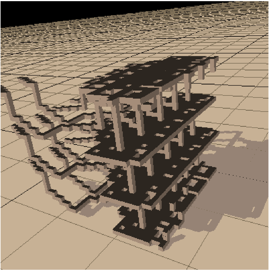
Figure 1: Visualization of an example brick “table” structure produced by GENRE.

Artificial development, also known as artificial embryology, is an area of artificial life that models biological processes of development, in which there are layers of abstraction between a genotype and a phenotype. The phenotype begins with a seed or embryo and progresses toward maturity according to a set of rules or interactions. The individuals on which evolutionary or other forces are acting are these processes by which the embryo develops. Developmental systems and other forms of indirect encodings of solutions can be contrasted with direct encodings, in which each component of the phenotype is made explicit in the genotype. As the problems being solved by evolutionary computation have grown in complexity, scalability has become an important aspect of the design of new evolutionary computation techniques, and certain properties of developmental systems, such as compact genotypes, lend themselves well to scalability (Bentley and Kumar, 1999; Hornby and Pollack, 2001a)as researched by Bentley and Kumar as well as Hornby and Pollack, which motivated much early research on artificial development (Tufte, 2008). A system that uses artificial development may be called a generative or developmental system.

Often, these developmental encodings are based on biological developmental processes and principles. Doursat (2009) used lower-level developmental processes such as cell division/differentiation and morphogen gradients to create a self-patterning “organic canvas,” and (Miller and Banzhaf, 2003)Miller and Banzhaf created a model for the programming of a cell, using cell division and simulated chemical environments, that was able to recreate a French flag and other patterns. Other approaches have involved the use of simulated gene regulatory networks (Guo et al., 2009), the exploitation of biological principles of degeneracy (Whitacre et al., 2010), and the evolution of grammars to generate programs or expressions in a given language (O’Neill and Ryan, 2001).

Below, we provide a brief overview of the two different generative systems used in this study.

GENRE

GENRE (Hornby and Pollack, 2001b) is a developmental system that was designed to create more complex virtual creatures than had been created using earlier artificial life techniques. It took a grammatical approach, evolving Lindenmayer systems (L-systems) (Lindenmayer, 1968), parallel grammatical rewriting rules originally designed to model plant growth, that took in parameters and would generate creatures with hundreds of components. The L-systems were applied iteratively to rewrite strings of commands through which to construct creatures or other structures, such that complex strings were constructed from simple ones. Hornby analogized the parallel nature of the rules, and the repetitive structures that they tended to produce, to concurrent cell division. The system outperformed a non-generative system on performance, creature size, and natural look, when applied to the design of mobile robots and block-based “table” structures. Hornby et al. 2001 observed that the generated robots appeared to exhibit modular properties, but did not attempt to quantify this. An example GENRE

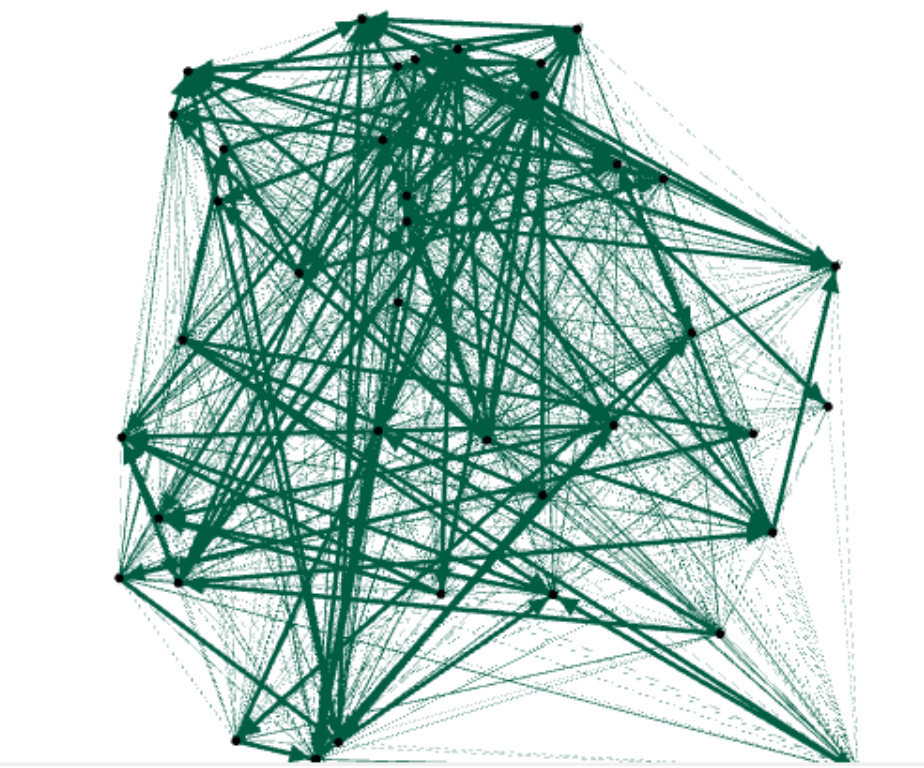
Figure 2: Visualization of an example artificial gene regulatory network (GRN) produced by GRNEAT.

produced structure can be seen in Fig.1.

GRNEAT

GRNEAT (Cussat-Blanc et al., 2015)Cussat-Blanc and colleagues, twenty-fifteen, evolves artificial gene regulatory networks, or GRNs (Banzhaf, 2003)Banzhaf, two-thousand three, which are simplified models of the genetic regulatory networks seen in biological systems, and used to control various kinds of agents. The GRNEAT algorithm evolves lists of proteins, which are then developed into network models with matrices of enhancing and inhibiting weights between nodes, mimicking the developmental module function of biological GRNs. The protein lists are used to initialize a GRN, which then updates its weights by calculating interactions between the proteins. It is based on NEAT (Stanley and Miikkulainen, 2002)Stanley and Miikkulainen, two-thousand two, a well-known algorithm for evolving neural networks, and retains NEAT’s major distinguishing features: initialization with small networks, a crossover operator that preserves subnetworks during GRN recombination, and the use of speciation to give growth opportunity to potentially promising innovations. However, a key difference is that artificial GRNs are inherently a developmental encoding, as biological gene regulatory networks are, while NEAT is a direct encoding algorithm. An example GRNEAT network, visualized in Gephi (Bastian et al., 2009)Bastian and colleagues, two-thousand nine, can be seen in Figure 2.

Methods

To test the effects of development on hierarchical modularity, we used the GENRE algorithm, which uses L-systems to model parallel cell division, and the GRNEAT algorithm, which evolves protein lists for construction of artificial gene regulatory networks in a manner mimicking NEAT’s neuroevolution methods, both of which are described briefly

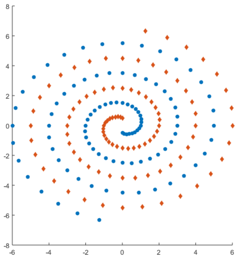
Figure 3: Illustration of two intertwining spirals, which must be distinguished from each other in the intertwining spirals problem.

above. We chose to compare GRNEAT to NEAT because, as stated above, GRNs are developmental by nature, so we could not simply compare a developmental GRN encoding to a nondevelopmental one. We ran GENRE on the bricktable-building problem that was one of its original test problems in (Hornby et al., 2001)Hornby and colleagues, two-thousand one, which rewards individuals for minimizing the number of bricks and maximixing height, surface area, volume, and stability, and compared the results to those obtained by a non-developmental evolutionary algorithm that is packaged with GENRE for the purpose of running comparisons. We ran the GRNEAT evolutionary process on the problem of distinguishing two intertwined spirals, also called the intertwined spirals problem (Lang, 1988)Lang, nineteen eighty-eight, which is illustrated in Figure 3, with fitness being measured by error ranging from -1 to 0, and compared the results to those obtained by running both feedforward and recurrent versions of the NEAT4J open source Java implementation of NEAT (Simmerson, 2006)Simmerson, two-thousand six, on the same problem.

Key parameters for GENRE and for GRNEAT/NEAT are listed in Table 1 and Table 2 respectively. While the comparisons between GRNEAT and NEAT were done primarily using simulations of 250 generations, we also did a set of runs of GRNEAT that were only 10 generations, to see whether any modularity that existed was actually emerging over time or was present early in the simulation. We did not do 10-generation runs for NEAT because it had made almost no progress at solving the intertwining spirals problem after only 10 generations. In the NEAT4J implementation

of NEAT, there is an option to allow or disallow recurrent neural networks. We decided to allow recurrency for a more even comparison, as GRNEAT produces recurrent networks. To prevent either the GRNs or neural networks simply memorizing a sequence of outputs rather than learning a mapping from coordinates to spiral ID, in both GRNEAT and NEAT, we used a fresh copy of the pre-initialized network for each new input.

Problem Version	Trials	Generations	Num R, P, C
GENRE	10	100	10, 2 , 2
Nongenerative	10	100	1, NA, NA

Table 1: Key parameters in GENRE experiments. R is the number of production rules, P is the number of parameters per rule, C is the number of condition-successor pairs per rule.

Problem Version	Trials	Generations	pC, pM, PopSize
GRNEAT	20	10	0.25, 0.75, 500
GRNEAT	20	250	0.25, 0.75, 500
NEAT	20	250	0.25, 0.75, 500

Table 2: Key parameters in GRNEAT experiments. pC is probability of crossover, pM is probability of mutation, PopSize is Population Size.

In order to look at the quantitative modularity of GENRE’s and its non-developmental counterpart’s brick table structures, we needed to represent the structures as networks. In order to do that, we defined each brick as a node, and each case of a face of one brick touching a face of another brick as a link. The link structure was binary, with all links being represented in the adjacency matrix as having a value of 1, and all other elements of the adjacency matrix having a value of zero. This was not necessary for GRNEAT/NEAT, as both GRNs and neural networks are already represented as networks, with links having non-binary weights. Since GRNEAT produces both a matrix of enhancement weights and a matrix of inhibition weights, we combined them into a single weight matrix by subtracting the inhibition factors from the enhancement factors.

Many artificial life and theoretical biology studies of modularity use the metric $Q$Q, defined by the approach of (Newman and Girvan, 2004)Newman and Girvan. This approach determines $Q$Q by looking at the percentage of edges in the network that connect nodes in the same module, and subtracts the expected value for that percentage in a network with the same number of modules but random connections. The modules are defined by a previous part of the algorithm that splits the network into the modules that would maximize $Q$Q. Mathematically, the equation for $Q$Q in the Newman-Girvan algorithm is:

$$Q=\sum _{s=1}^k\left[\frac{l_s}{L}-{\left(\frac{d_s}{2L}\right)}^2\right]\text{\hspace{1em}(1)}$$

Q is defined as the sum from s equals one to k, of the quantity, l sub s over L, minus the square of the quantity, d sub s over two L

where $L$L is the number of edges, $K$K is the number of modules, $d_s$d sub s is the sum of degrees of nodes in module $s$s, and $l_s$l sub s is the number of edges in that module.

This method is very useful for examining a single layer of modularity in binary networks (i.e. networks where there is either a connection between two nodes or there is not). However, the weights of links between nodes in GRNs can vary by several orders of magnitude. Both GRNs and recurrent neural networks may benefit from a modularity metric that can account for directedness. And the Newman-Girvan approach only looks for one layer of modularity, rather than for hierarchical modularity. Accordingly, we used the “Louvain method,” which was designed for speed, maximization of community detection, and the detection of hierarchical levels of modularity, to determine $Q$ (Blondel et al., 2008)Blondel and colleagues. In the Louvain method, each node in the network is initially assigned to its own module, and the modularity $Q$Q is calculated according to the following equation for a weighted graph:

$$Q=\frac{1}{2m}\sum _{i,j}\left[A_{ij}-\frac{k_i{k}_j}{2m}\right]\delta (c_i,c_j)\text{\hspace{1em}(2)}$$

Q equals one over two m, times the sum over i and j, of the quantity, A sub i j minus k i k j over two m, all multiplied by the delta function of c i and c j

where $A_{ij}$A sub i j represents edge weight between nodes $i$i and $j$j, $m$m represents half the sum of the graph’s edge weights, $\delta$delta is a delta function, $c_i$c sub i and $c_j$c sub j are node communities, and $k_i$k sub i and $k_j$k sub j are the sums of the weights of all edges attached to node $i$i and node $j$j respectively.

Then, for each node, the algorithm calculates the change in modularity, the equation for which depends on whether the version of the algorithm for directed or undirected graphs is being used, for moving that node into the module of each of its neighbors. Once this change is calculated for all modules that the node is connected to, the node is moved into the module that would result in the greatest modularity increase (or left in place if no modularity increase is possible). If no increase is possible, the first level of $Q$Q is equal to the current modularity of the network. Subsequent, hierarchical levels of $Q$Q are calculated the same way in subsequent phases of the algorithm, by using the modules from the previous level as nodes in a new network. For our study, we used Antoine Scherrer’s MATLAB implementation of the Louvain method (Scherrer, 2008)as implemented by Scherrer.

Because modularity can be positive or negative (where negative modularity means that there is less internal integration among modules than one would expect to see in a random graph), we defined a level of modularity as occurring when the Louvain algorithm produces a positive modularity

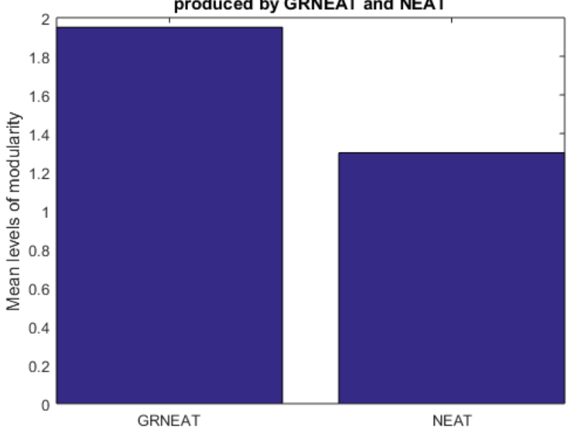
Figure 4: The mean number of levels of hierarchical modularity produced by a developmental network-evolving system, GRNEAT, was higher than that produced by the non-developmental one on which it is based, NEAT. The 95% CIs for GRNEAT and NEAT were 1.85-2.05 and 1.09-1.51. Number of trials $N=20$N equals twenty, $p<0.0001$p less than zero point zero zero zero one

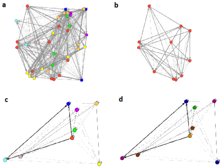
Figure 5: a) A GRNEAT-produced GRN with the links lightened for easier viewing. The nodes are colored according to the 8 first-level modules found by the first phase of the Louvain algorithm, which found that this level of modularity had $Q=0.3018$Q equals zero point three zero one eight. b) A single module of the GRN. c) The network of the next level of hierarchy, with each of its node representing, and color-coded as, a module from the previous level. d) The same next-level network, with $Q=0.3266$Q equals zero point three two six six, with the nodes colored in five new colors according to the 5 second-level modules found by the second phase of the Louvain algorithm.

value, with an allocation of nodes into modules that (if there are lower levels) involves combining some or all modules from the next-lowest level. To determine whether the numbers of hierarchical levels of Louvain modularity were equal in our sets of results, we used Welch’s t-test, a variant of the traditional Student’s t-test that is robust to non-normality in data and difference in variance between samples. We did not test for differences in the actual $Q$Q values of the lowest or other levels, as they were tangential to the question of hierarchy. In practice, $Q$Q values for specific levels were between 0.12 and 0.52 for both GRNEAT and NEAT (with most being between 0.2 and 0.4, indicating moderate amounts of single-level modularity), and between 0.3 and 0.72 for both GENRE and its direct encoding counterpart.

Results and Discussion

Our first comparisons were between a set of 20 trials of GRNEAT on the intertwined sprials problem and 20 trials of NEAT with recurrency allowed on the intertwined sprials problem, with mutation probability = 0.75 and crossover probability = 0.25, across 250 generations. In Figure 4, we can see that the best solutions produced in the GRNEAT trials had a mean number of levels of modularity of 1.95, while those produced in the NEAT trials had a mean number of levels of modularity of 1.3, a full 33% lower. This difference in the means was statisically significant ($p<0.0001$)with a p value less than zero point zero zero zero one. The emergence of multiple levels of modularity in one GRN is shown in Figure 5.

We wanted to examine whether the increased levels of modularity seen in GRNEAT were something that was emerging rather than something hard-coded into all GRNs.

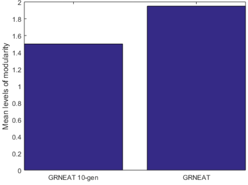
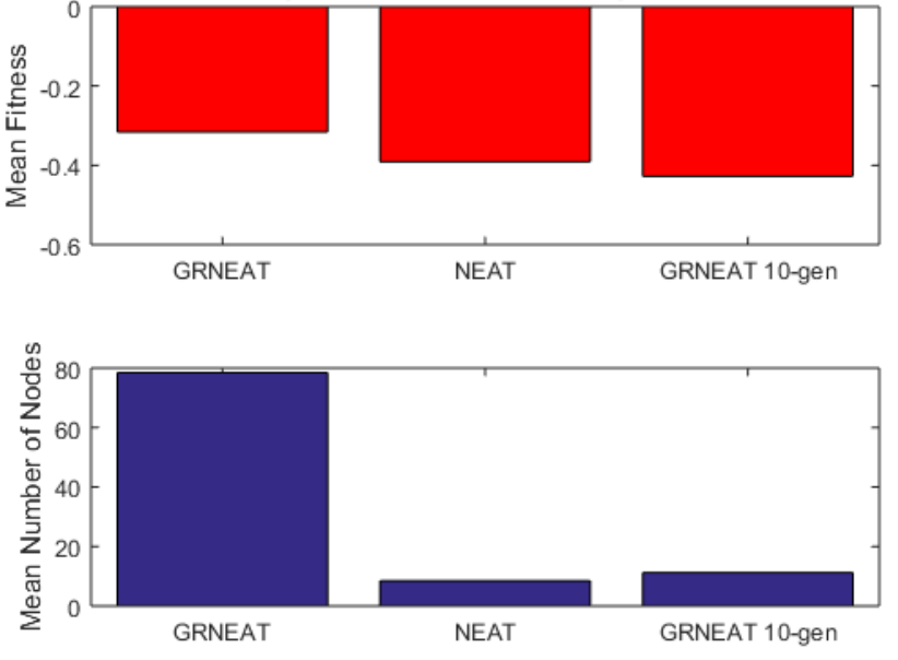
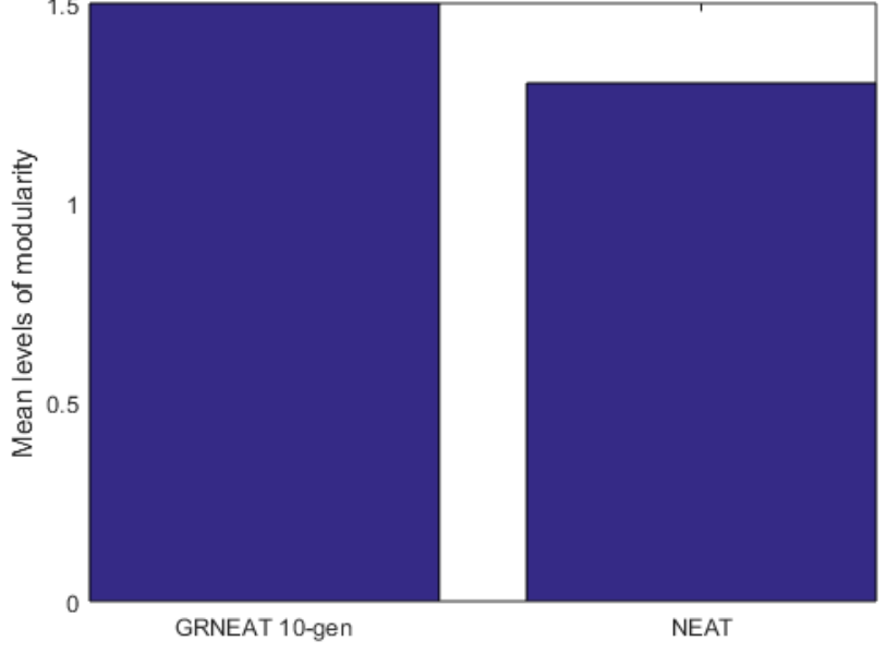
Because the average fitness of the NEAT neural networks after 250 generations was notably worse than that of the GRNEAT GRNs, and the networks notably smaller (see Fig.6), we also wanted to compare the NEAT networks to GRNs of more similar fitness and size. Accordingly, we compared the 20 250-generation GRNEAT trials to 20 10-generation trials (Fig.7), and, as the 10-generation GRNEAT GRNs were similar in size and fitness to the NEAT neural networks, we compared the 10-generation GRNEAT trials to the NEAT trials (Fig.8).

We can see from these figures that the mean hierarchical modularity of GRNEAT-produced GRNs (along with the size) has increased by nearly a third (a mean 1.5 levels of modularity vs 1.95 levels) between the 10th and 250th generations. We can also see tentative evidence (with a $p$p value that is low but not statistically significant) that GRNEAT GRNs already have greater hierarchical modularity after 10 generations than NEAT recurrent neural networks have after 250, despite being nearly the same size, which is suggestive that this increased hierarchy is not solely a function of network size.

While the most obvious difference between GRNEAT and NEAT is the artificial development aspect, it is possible that there is some other factor influencing the development of hierarchical modularity. Therefore, we looked at a different developmental system using a very different

Figure 6: 250 generations of GRNEAT produced top solutions with greater mean fitness than 250 generations of NEAT. 250 generations of NEAT still had greater fitness than 10 generations of GRNEAT.

Figure 7: Networks produced by GRNEAT after 250 generations had greater mean levels of hierarchical modularity than networks produced by GRNEAT after 10 generations. The 95% CIs for GRNEAT and 10-generation GRNEAT were 1.85-2.05 and 1.28-1.72. Number of trials $N=20,p=0.0014$N equals 20, p equals 0.0014

mechanism of development, GENRE, and compared it to the direct encoding algorithm packaged with its implementation on the GENRE homepage (Hornby, 2001), as discussed in the Methods section. One useful aspect of looking at GENRE’s brick-table structures is that the default fitness function for these structures encourages minimizing the number of blocks while maximizing other structural criteria. While, because of the nature of the block structures, the GENRE network representations were much larger than the GRNEAT or NEAT representations, they were actually smaller than those of the direct encoding alternative (640 blocks vs 768 blocks). Therefore, the possibility of network size being a major contributor to the different levels of hierarchy produced by a developmental vs a direct encoding is addressed.

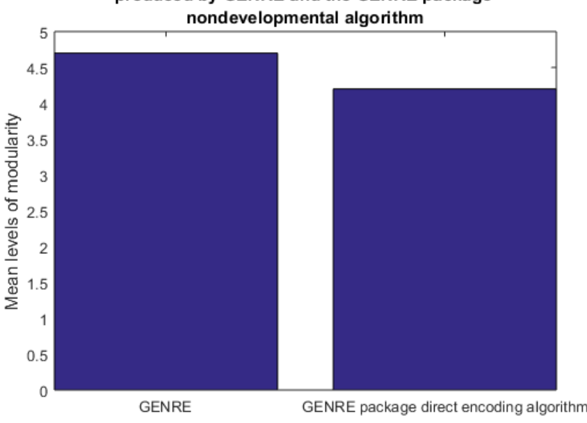
As can be seen in Fig.9, there is a statistically significant ($p=0.0246$p equals 0.0246) difference between the levels of hierarchical modularity produced by GENRE as compared to its nondevelopmental alternative, where the GENRE-produced structures had an average of 4.7 levels, and the others had an average of 4.2.

Notably, in both cases, the number of levels was far higher than for GRNEAT or NEAT, regardless of development, and the network sizes were much larger, which suggests that network size may play some role in the number of levels of hierarchical modularity. However, the fact that GENRE structures have more levels than do a nondevelopmental algorithm optimizing for the same fitness function, in the same number of generations, despite being 17% smaller, provides further evidence that the developmental encoding is doing some of the work in the emergence of this hierarchy.

Conclusion and Future Work

This work opens up two different areas of study. One is the study of the effects of developmental encodings on the emergence of modularity. This is an underexplored area, with the potential to contribute to our understading of the emergence of modularity in general. To our knowledge, this is the first time that developmental encoding effects on the emergence of modularity have been quantified. Another is the study of hierarchical modularity. While modularity is an active area of research, as we outlined earlier in this paper, the hierarchical aspect of modularity has been ignored in modularity-emergence studies despite the importance of hierarchy in biological and other understandings of modularity. This paper takes a first step toward remedying this oversight.

Our results suggest several more specific avenues for future work. It may be useful to compare other developmental systems to similar nondevelopmental ones, to see whether the same effect is observed. Even though GENRE and GRNEAT use very different mechanisms for encoding development, increasing the number of systems studied may provide more evidence that the effect seen here is mechanism-independent. Another possibility would be to adjust different parameters within the developmental systems, to see if other factors can be identified that promote the emergence of hierarchical modularity. Finally, it would be interesting to study the effects of development in biological systems, as was done in (Kashtan et al., 2007; Parter et al., 2007)Kashtan and colleagues, and Parter and colleagues to determine the effect of varying goals on modularity.

Figure 8: The mean number of levels of hierarchical modularity produced by only 10 generations of GRNEAT was higher than that produced by 250 generations of NEAT. The 95% CIs for 10-generation GRNEAT and NEAT were 1.28-1.72 and 1.09-1.51. Number of trials $N=20,p=0.2$

Figure 9: The mean number of levels of hierarchical modularity produced by a developmental brick-table-evolving algorithm, GENRE, was higher than that produced by the nondevelopmental algorithm with which it is packaged. The 95% CIs for GENRE and the nondevelopmental algorithm were 4.4-5.0 and 3.94-4.46. Number of trials $N=10,p=0.0246$

Acknowledgments.

Many thanks to Kyle Harrington for his help in troubleshooting GRNEAT and other code and his valuable feedback.

References

[references omitted]

[references omitted]