Emergent Models: Intelligence from Tiny Substrates
Giacomo Bocchese, Nicola Giacobbo, Etienne Guichard, James Wiles, Akshaj Devireddy
Wolfram Institute, Emergent Computing, Østfold University College
Abstract
Emergent Models (EMs) are a machine learning paradigm based on simple yet open-ended substrates, such as cellular automata, in which modeling is treated not as the learning of a closed-form input-output map but as the emergence, within simple dynamical systems, of computational behaviors that solve external tasks. Such substrates typically iterate a fixed local rule over a latent space for an adaptive number of steps, with an interface linking the latent state to external input/output signals. Training proceeds by evolutionary search. We hypothesize that some instances of this framework are biased toward global generalization: capturing the rule generating the data over its full domain, and therefore extrapolating beyond the training range. Theoretically, we prove that some EMs are latent-universal: with the update rule and interface held fixed, they can realize any partial computable function by varying only the initial condition of the latent state. Empirically, we study a zoo of minimal EM instantiations across discrete and continuous substrates, showing that local-recursive computation at a tiny scale (tens to hundreds of parameters) can extrapolate exactly on simple arithmetic functions, can support control behaviour and online adaptation, while still exposing several limitations. This work is foundational: it does not propose a competitive architecture, but a framework meant to widen the design space of machine learning beyond differentiable feed-forward maps.
1 Introduction
Sutton’s “Bitter Lesson” argues that the strongest long-run progress in AI comes from general methods that leverage compute, rather than from direct top-down engineering
Emergent Models (EMs) formalize this perspective by turning such dynamical systems into machine learning models, coupled to external inputs and outputs through an encoding and decoding interface.
But which notion of openness is relevant for machine learning? And is there a precondition for a substrate to “leverage compute”? We argue that both questions have the same answer: expressivity, the set of functions a model can theoretically represent. Search can only select among functions a model can express: a target behavior outside this range is unreachable at any compute budget.
Because the term expressivity is often used informally and varies across contexts
Much of traditional deep learning is based on feed-forward neural networks (FFNNs)
In traditional recurrent or autoregressive architectures, such as standard (non-reasoning) RNNs and Transformers,
each datapoint prediction is obtained through a single forward pass
This raises a question about compression: how small can the iterated update function be while still supporting high global expressivity, and does smallness itself carry favorable inductive biases for extrapolation? Compact recursive models such as Hierarchical Reasoning Models (HRMs) and Tiny Recursive Models (TRMs) match mid-size LLMs on ARC-AGI-style reasoning with
The emphasis on iteration is grounded in computation theory: in classical models of computation (eg. Turing machines), complex algorithmic behavior arises from repeatedly applying simple update rules to a mutable memory state, with computation time and memory allowed to vary depending on input and task complexity. Looping is not an implementation detail, but one of the core ingredients that makes general computation possible
Cellular automata (CAs) are a natural substrate in this setting. They combine a simple local rule with iterative dynamics over a potentially unbounded medium, and some, including Conway’s Game of Life and Rule 110, are Turing complete
The use of CAs in machine learning is not entirely new, and so far has followed two main approaches: CA reservoirs and NCAs. Reservoir methods treat the automaton as a fixed dynamical medium and train only an external linear readout of its trajectories
In this work, we formalize this perspective through a framework that turns dynamical systems into machine learning models. In its strongest ideal regime, which we call latent universality (theorem 1), the update rule is fixed and varying only the initial state suffices to express any computable function.
Our experiments deliberately study a simpler setting: they do not realize latent universality, and no experimental claim depends on Theorem 1. Rather than fine-tuning a single construction toward the full theory, we examine a zoo of minimal Emergent Model instantiations to convey the idea and philosophy behind the framework, as befits the opening stage of this research. These show that local-recursive modeling at a tiny scale (20-300 parameters) can extrapolate on simple arithmetic functions and can produce control behaviors, indicating that such substrates are meaningful in principle, not that they are easy to train or competitive with mature task-specific methods.
2 Emergent Models
2.1 Intuition
A broad class of latent-space reasoning models can be summarized schematically as:
where a fixed update function
into the latent space, and the decoder
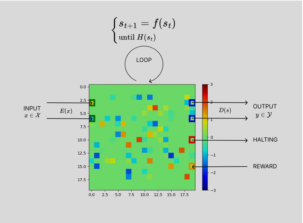
Figure 1 shows a didactical instance: a continuous two-dimensional lattice with an interface based on fixed cell positions: inputs and outputs are written and read at designated locations (ports).
Both the latent state and the interface admit far more general forms than this example. The latent state may be unbounded in space, as in a Turing machine tape,
Emergent Models formalize this picture through a generalized automaton: a discrete-time dynamical system with a halting condition. Equipping the automaton with an interface (encoder and decoder) turns the dynamical system into a model. The following subsections make this construction mathematically rigorous.
2.2 Generalised Automaton
The topology of the latent state space
Let
Each node of the graph carries a value in a set
The edges define the neighborhood structure, but do not play a direct role in the formalism, as explained below.
Typical choices are (i) a one-dimensional unbounded tape, as in Turing machines or 1-d CAs, with and finite alphabet , or (ii) a two-dimensional finite
lattice, with
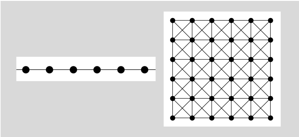
A transition function
The transition function is local if there exists a function such that for every and every vertex ,
The transition function can be realized in many ways, such as lookup tables in discrete cellular automata, neural networks in neural cellular automata, polynomial maps, and other computable rules.
A generalized automaton is a tuple that, starting from an initial condition , generates a trajectory and, if halting occurs, terminates at a state . Many computational devices can be abstracted in this way, including Finite State Machines, Turing machines
2.3 The model
An Emergent Model is a tuple
Let be an encoder function, mapping from an input space into the latent space , and let be a decoder, reading an output in from the latent space .
The automaton starts from a non-perturbed () initial state , which we call the program. Given an input , the encoder produces a state . The actual (perturbed) initial state is then obtained by combining the program with the encoded input:
where is a simple total computable combining operator, typically given by sum, overwrite at particular locations or similar operations.
From this point on, program always indicates the non-perturbed initial state, while initial state refers to the perturbed initial state . An example construction of the initial state by combination is shown in fig. 4.
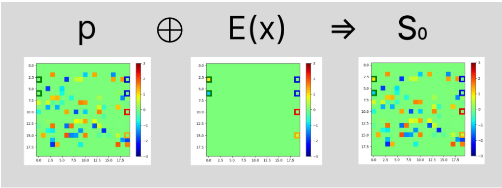
The program should not be understood as a symbolic algorithm explicitly compiled into the substrate, as in a programming language. It is instead a raw substrate-level configuration: a pattern in the state space that conditions the system’s evolution so as to induce a particular function. In this sense it still captures what we take to be the essence of a program (a state held in memory that steers the computation) but without the symbolic, human-written form that word usually implies.
Inference proceeds as follows: initialize the state with the program, encode the input, run the dynamics
whenever the halting time
In machine learning, a model is treated as a parametrized function
Modeling then means finding parameters
Definition 1 (Model computes a function). Let
If
and is undefined for .
If
The tolerance
Which functions a model can compute depends on both the substrate and the parametrization chosen. Different substrates and parametrizations therefore compute different classes of functions, presenting different degrees of expressivity. The maximal degree in the computational setting is Turing completeness, or computational universality: a single model able to represent every partial computable function by varying
We theorize a special regime, called latent universality (Section 2.4), in which the transition function, state space topology, and interface are all fixed and the program alone determines the computation the model performs (). In this regime, taking and
The encoder and decoder must be simple, total computable, and compatible with the dynamics of the chosen automaton
2.4 Latent Universality
Assuming the input/output spaces are binary strings
Latent universality is not meant as a new universality claim at the level of computability theory, but as a reformulation of it in natural terms for machine learning on dynamical systems. In Universal Turing Machines
The analogy should not be interpreted as requiring a compiler from symbolic algorithms to substrate programs: the program is treated as a trainable substrate-level variable, and learning consists of searching over raw program states that induce the desired behavior when paired with inputs. Inputs, by contrast, may be compiled: the encoder syntactically transforms them into a fixed representation the machine can read, with no information about the program nor about the target function to be realized. This asymmetry is what motivates keeping the program and the encoded input separate and combining them afterwards, rather than compiling both jointly through a single map : since the encoder acts only on and not on , any program can be searched while inputs are presented to the substrate through a common, fixed interface. This formulation departs slightly from the standard pairing convention, which does not generally require program and input to be separable; several known universal
Turing machines nonetheless admit this disjoint form, initializing the tape with the simulated machine description and the encoded input in distinct regions or tapes, with no interdependence between the two: the encoder of
We work in a strong-universality setting. The substrate has an unbounded topology (countably infinite
Theorem 1 (Latent Universality). Let
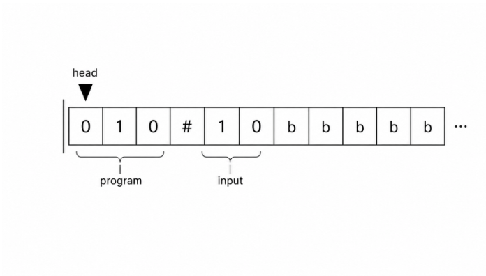
In
Using
On a one-sided, one-dimensional tape (
The same structure extends beyond tapes. On a two-dimensional grid, the program and the encoded input are both full-grid states, each non-quiescent only on its own finite region, and
The flexibility of the paradigm leaves open further constructions: with a continuous value set
2.5 Sequential Operation, State Retention and Meta Learning
So far, the EM formalism defines a predictor acting on a single input,
A naive rule to pass information to the next macrostep would be to set the next program equal to the previous terminal state,
The operator
For example, in a Turing Machine,
a reset is valid only if the retained state does not prevent the machine from starting and performing the next computation correctly. Retention may require a substrate and interface designed so that persistent memory can coexist with repeated computation and not every latent-universal construction is necessarily compatible with this regime.
The program at first macrostep is initialized as
In control or reinforcement-learning settings, it is natural to augment each macrostep input with reward information, writing
Retained state is not merely passive memory. Because each new computation starts from the retained program , the stream of inputs can influence the future computation itself. In latent-universal settings, universality implies that the substrate can in principle represent any algorithm, while the latent nature of the program makes that algorithm part of the mutable state itself, suggesting the following conjecture: given sufficient memory and computation time, and providing the reward as an input, there exist some EMs that implement internally: (i) a prediction subroutine, which maps the current input to an output, and (ii) an update subroutine, which uses reward signal to modify a designated sub-portion of the program. In this view, the model could not only execute a prediction but also a feedback-driven self-improvement procedure acting on its own latent program, realizing a form of meta-learning
2.6 Extensions and Relaxations
The Emergent Model theoretical framework extends naturally to continuous-time dynamical systems, and in particular to continuous media governed by local field dynamics.
At the most general level, one may replace the discrete transition with a continuous-time evolution law:
This ODE form is an abstract state-space description and does not, by itself, impose any notion of locality. A more structured extension is obtained when the state is a field over an Euclidean spatial domain
where the
This yields a natural notion of continuous-space computation, encompassing substrates such as reaction-diffusion systems and other fluid-like media.
Under these extensions, the interface formalism remains unchanged: the encoder , decoder , halting , and combining operator are still defined as maps on the state space. The halting time is defined analogously as:
whenever this quantity exists and is finite.
Another natural relaxation is allowing stochastic evolution rules, where the dynamics include random fluctuations or noise, so the same initial state may generate different trajectories. The induced output is then stochastic.
A more practical relaxation is to cap, or even fix the internal computation time. Instead of running the dynamics until an explicit halting condition is met, one may apply the transition rule for a fixed time budget . This reduces expressivity but also removes the possibility of non-halting predictions, makes inference easier to parallelize on hardware, and can simplify state retention. Under suitable conditions, this allows identity state retention
A further, mostly notational relaxation is to reframe the state initialization in pseudocode. Instead of explicitly forming , one practically sets the initial state as the program and then overwrites the encoded input into a designated subspace:
s0 <- p
I <- InputSubspace(s0, x)
s0[I] <- E(x)
Here s0[I] <- E(x) represents an overwrite operation that injects the encoded input into that region, while the rest of
For example, if the state space is a vector and the input is
s0 <- p
s0[2:4] <- [x1, x2]
Under this procedural view, an Emergent Model can be represented in pseudocode as follows.
For non-sequential tasks, without retention, a single prediction is:
Input x
Program p

s <- p
I <- InputSubspace(s, x)
s[I] <- E(x)
for t in microsteps do
  s <- f(s)
y <- D(s)
On sequential tasks, with retention:
Input stream (x_i)_{i in macrosteps}
Program p

s <- p
for i in macrosteps do
  I <- InputSubspace(s, x_i)
  s[I] <- E(x_i)
  for t in microsteps do
	s <- f(s)
  y_i <- D(s)
  s <- R(s)
2.7 Training
After choosing which components are trainable, optimizing an Emergent Model means searching for configurations that make the induced computation solve a desired task. In supervised settings, this amounts to minimizing a prediction error; in control and reinforcement-learning settings, to maximizing expected cumulative reward
Let
while in control tasks we solve:
In the most general case,
In latent-universal settings only the soft parameters are trained for a particular task, while the hard ones
Crucially, the search is guided only by the decoded output: the intermediate microstep trajectory
Although many training algorithms can be employed, EM dynamics are strongly recursive, nonconvex, and often discrete, making gradient-based methods impractical or impossible to use. Evolutionary algorithms are therefore a natural choice, especially in the most open-ended scenarios. In latent-universal settings, any computable function is realized by some finite-support initial state
Lemma 1 (Searchability)
Let
M be latent universal and assume programs are finite-support states, i.e. withp is a finite string rho in the set of all binary strings followed by an infinite background . Then for every partial computable functiong from binary strings to binary strings there exists such a finite stringrho sub g that allows the computation of . In particular, since is countable, enumerating programs (or sampling them at random with variable length) will eventually hit a program that computes .
The searchability lemma clarifies why finite-support programs are essential for treating latent-universal EMs as machine-learning models. If the target program has finite support, then it can be searched by enumeration, random sampling or by a finite sequence of edits (insertions, deletions, mutations). In this sense, EM training is viewed as emergent program synthesis: rather than designing an algorithm at a high level and compiling it into the substrate, one searches over substrate-level initial states until a configuration inducing the desired behavior is found. The lemma provides only an asymptotic existence condition: a suitable program exists and is reachable in principle, but the search may be arbitrarily long and no efficiency guarantee is implied.
3 Experiments
The experiments described below are intended to validate the Emergent Model framework and demonstrate it is non-vacuous, rather than to benchmark it against optimized task-specific approaches. None of the tested substrate-interface combinations is shown to be latent-universal; we favor evaluating a broad zoo of minimal models over engineering one toward the full theory. The goal is to test whether simple physical-like substrates, equipped with minimal input-output interfaces and trained by evolutionary search, can exhibit use-
ful modeling capabilities, extrapolation, control, and adaptation.
Across experiments, we use generational population-based genetic algorithms (GAs) to optimize each model’s trainable components, such as program state, transition-rule parameters, or interface parameters. Each generation evaluates candidate models, selects high-performing individuals through tournament selection, and forms the next population through elitism, sparse crossover, and mutation. This provides a simple black-box training method for discrete, non-differentiable, and strongly recurrent substrates. The exact GA variant and fitness objective vary slightly across tasks, and we report representative training and evaluation runs rather than full multi-seed statistical analyses. In some control experiments, we apply state retention across macrosteps, episodes, and generations, so that inference and environment interactions modify the latent state that will be reused in subsequent evaluations. Thus the soft parameters are updated by the model’s own dynamics and interaction history. When a parent is selected, crossover and mutation are applied only to its hard parameters, while its final latent state is copied directly to the offspring. We refer to this convention as Lamarckian-style state inheritance: advantageous state changes can be inherited, even though the state is mutated by inference dynamics rather than by external noise.
The experiments are organized by task family: Arithmetic tasks test exact rule learning and extrapolation in discrete domains; CartPole tests simple closed-loop control; and Meta-Life tests a more complex control objective, with online policy adaptation.
3.1 Arithmetic tasks
We first evaluate Emergent Models on simple integer arithmetic tasks. Arithmetics is a natural test case for this framework because it requires learning an exact symbolic rule and extrapolating beyond the finite training range. Discrete local cellular automata are especially well suited to this setting, where inputs and outputs are integers, and computation can be represented through spatial interactions over a discrete latent state.
The learned program is fixed across datapoints of a task. For each input, the automaton is reinitialized from the program, then the input is encoded into the state, and the system is run until halting. No terminal state is retained, since these are non-sequential regression tasks.
3.2 EM43
We ran minimal experiments to test whether EM43, an Emergent Model made from a minimal discrete cellular automata, can learn simple arithmetic functions and extrapolate far beyond the training range. Training is performed jointly on the program and the rule for each of the following tasks:
EM43 is a one-dimensional cellular automaton with one-sided tape, radius
Given a global automaton state
The tape at initial state
The present setting was adopted as a largely arbitrary, minimally engineered design. It should therefore be regarded as one among many possible automaton-interface combinations, and more effective ones may exist.
Training is performed on inputs in
The learning algorithm is a generational island-based ge-
netic algorithm with tournament selection, pointwise mutation, crossover, elitism, and island migration
Fitness
where
For each task, independent training runs are performed using a fixed population of 20 islands with 2000 individuals each (40000 total), and a number of generations increasing with task complexity. The parametrization consists of a trainable program of length
3.2.1 Results
After training, exact-match accuracy is evaluated on the training and test sets and averaged over runs. Table 1 summarizes the results.
| task | runs | gens | params | bits | train acc | test acc | |
|---|---|---|---|---|---|---|---|
| 8 | 20 | 10 | 70 | 140 | 100% | 100% | |
| 8 | 90 | 10 | 70 | 140 | 100% | 100% | |
| 8 | 150 | 10 | 70 | 140 | 100% | 100% | |
| 8 | 400 | 10 | 70 | 140 | 100% | 100% | |
| 2 | 500 | 10 | 70 | 140 | 100% | 100% | |
| 2 | 800 | 50 | 110 | 220 | <20% | <10% |
Table 1: Performance of EM43 across different tasks, showing number of runs, generations, parameter size, and accuracy.
Perfect extrapolation is observed, in all runs, for all one-input tasks considered. This behavior is especially notable for periodic functions such as
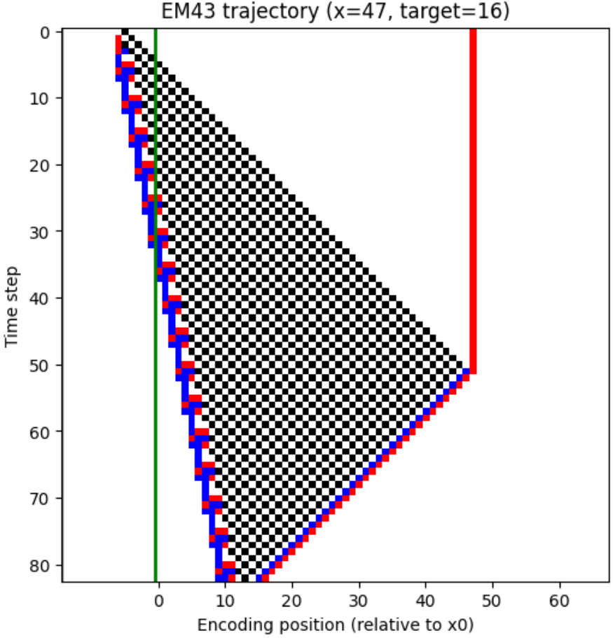
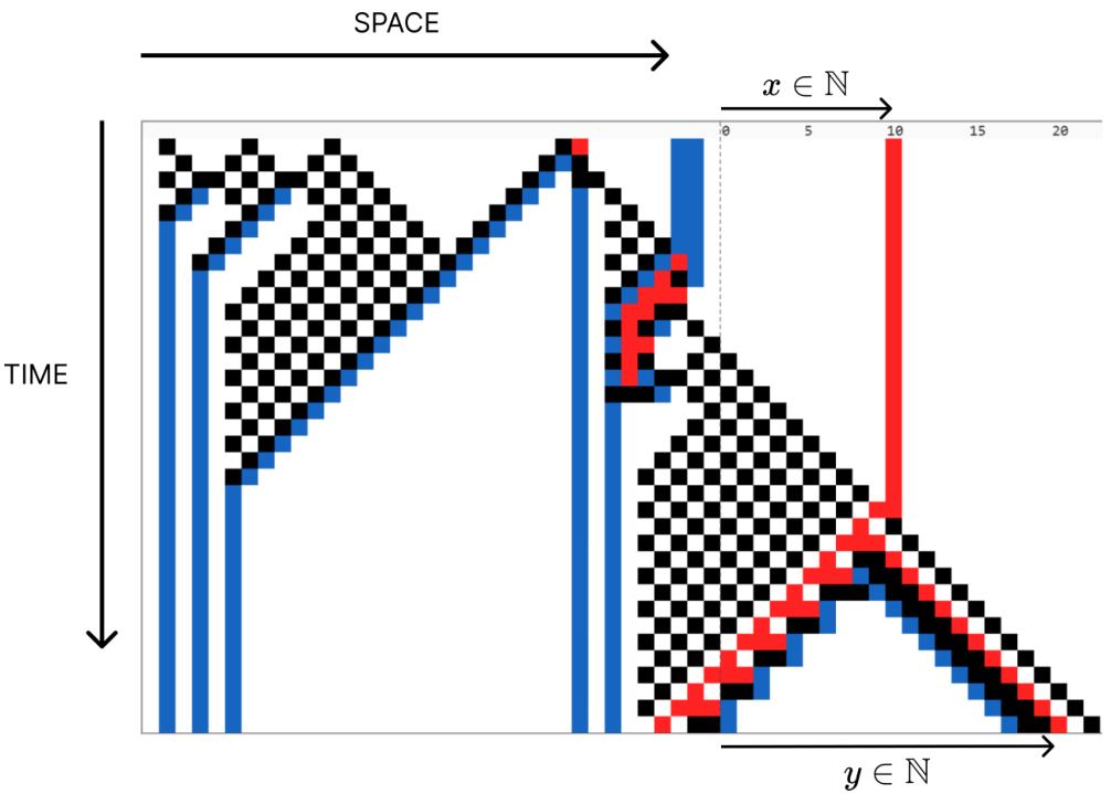
Plotting the space-time diagrams of configurations that generalize reveals an interesting phenomenon that we call geometric grokking: exact computation is typically carried by regular and interpretable geometric patterns that remain stable across input scales. In the case of
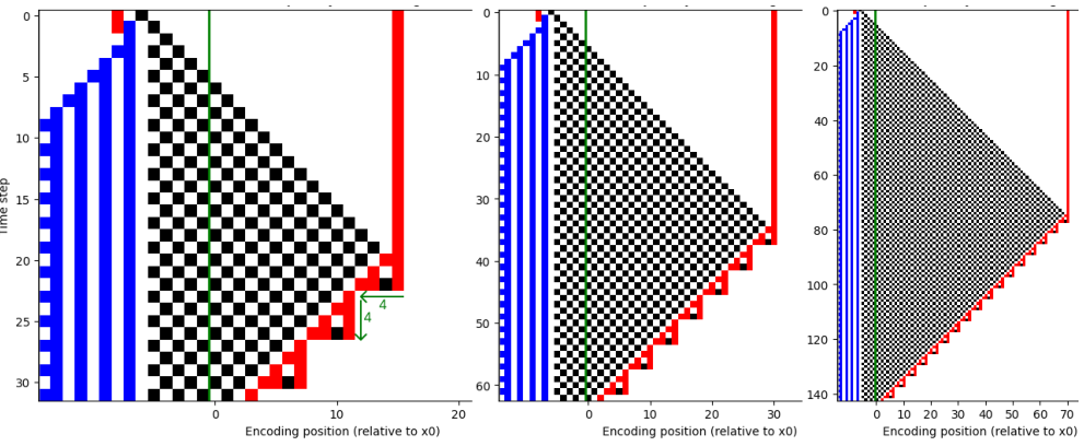
The task
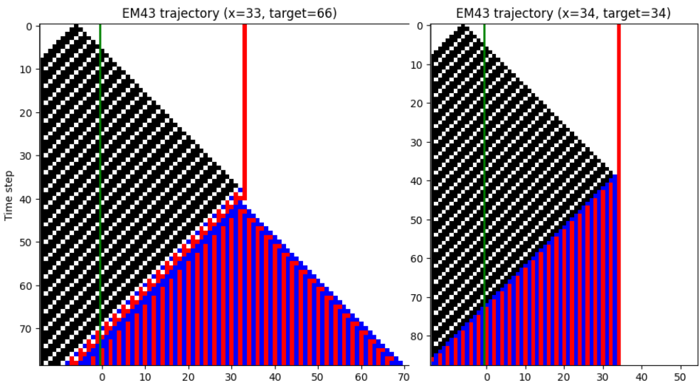
Different runs and tasks implement different geometric strategies, but they typically follow the same broad scheme: patterns propagate from the program region, collide with the input marker, and eventually trigger halting through changes in the active-cell population
More complex tasks such as
A notable aspect of this setting is the small size: 70 parameters carrying 2 bits each, corresponding to 140 bits of information. The setup is also data-efficient, being trained on only 30 integer examples while extrapolating to much larger ranges. This combination of parameter and data efficiency is broadly consistent with observations in the Neural Cellular Automata literature
3.3 GoL-EM
We next test the EM framework in Conway’s Game of Life (GoL) on simple arithmetic tasks. The GoL rule is fixed, and training acts only on initial conditions. This matches the latent-program view from Section 2.4: task-specific computation is encoded in the initial condition, not in the transition rule.
However, GoL’s Turing completeness does not automatically transfer to this setup. Indeed the chosen input encoding, output decoding, and halting protocol can restrict access to universal constructions. Since our interface and halting policy is deliberately minimal and not proven to preserve universality, this experiment should be read as a small-scale test of initial-state optimization in a fixed cellular-automaton substrate, not as a demonstration of latent universality.
3.3.1 Methodology
We use a square GoL board as a fixed computational substrate. The automaton is binary-valued: 1 denotes a live cell and 0 denotes a dead cell, so the value set is
The board is partitioned along each axis into three consecutive regions: the program region of side
To reduce the search burden, we do not optimize over arbitrary live/dead patterns in the program region; instead, we search over glider placements, using the upper-left corner
of each glider as a trainable position variable. These gliders travel towards the input region and eventually interact with the encoded inputs.
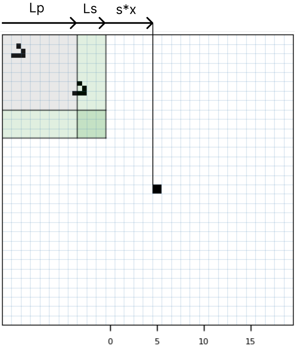
Inputs are encoded positionally, on the diagonal of the encoding region. For an input value
The state then evolves under the standard Conway’s GoL update rule. Computation halts when the system reaches equilibrium/fixed point:
At halting, the output is decoded by scanning the encoding region for isolated live blocks. Among all valid candidates, the leftmost block is selected, and its horizontal position relative to the encoding origin is converted back into a scalar using the same stride as in the input encoding. Unlike input, output blocks are not required to lie on the diagonal: only their horizontal position is used. Moreover, other live-cell debris that may remain elsewhere on the board is ignored by the decoder. This gives the dynamics more freedom to form a valid output and reduces the search burden.
Let
During training, if the halting condition is not reached within a maximum time budget
We train the GoL program by minimizing prediction error while penalizing invalid computations:
Here is the mean absolute error on the training dataset, and is the fraction of examples that failed to produce a valid prediction. This includes both non-halting runs and halted runs with no decodable output block.
We optimize the program with two black-box search methods over glider positions in the program region: a genetic algorithm with mutation on glider positions, and plain random search that samples positions uniformly. The two reach almost identical results, so we report random search throughout, being the simpler. This near-equivalence is itself informative about the search landscape, and we return to it below.
3.3.2 Results
The GoL model successfully learned and generalized tasks of the family
| task | train dataset | test dataset |
|---|---|---|
| , even , odd |
Table 2: Training and evaluation input ranges for GoL arithmetic tasks. Lower bounds are chosen so that the target output is non-negative, since the positional decoder is not designed to represent negative integers.
| task | train acc | test acc | |||
|---|---|---|---|---|---|
| 40k | 2 | 18 | 100% | 100% | |
| 40k | 2 | 18 | 100% | 100% | |
| 40k | 2 | 18 | 100% | 100% | |
| 40k | 2 | 18 | 100% | 100% | |
| 40k | 2 | 18 | 100% | 100% | |
| even odd | 1M | 3 | 26 | 60% | 50% |
Table 3: Performance of the GoL-based Emergent Model across tested tasks, trained by random search over glider positions.
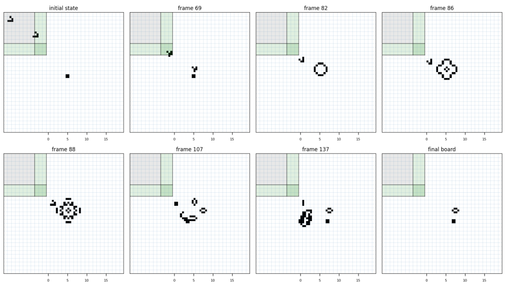
Several limitations remain. First, although GoL itself is universal under proper constructions
3.4 Control tasks
We next evaluate some Emergent Models in control settings. Differently from arithmetic tasks, the goal here is not extrapolation over unbounded ranges: observations and actions are typically bounded by the environment. Instead, it tests whether a simple substrate can support closed-loop behavior and robustness.
State retention becomes more relevant in this setting, because the controller acts on a stream of observations rather than on isolated datapoints. Instead, adaptive computation time through explicit halting is less central here than in static arithmetic tasks: in a control loop, computation is already distributed across macrosteps, since each new observation triggers another round of internal updates. For this reason, some of the controllers below use a fixed computation time budget
We consider two environments. The first is CartPole, a standard continuous-state control task in which the agent must balance a pole by applying forces to a cart. The second is Meta-Life, a simple 2-d spatial navigation and foraging environment, which we study in two variants: Meta-Life-Food, where agents learn to move and collect food, and Meta-Life-Adapt, where resources alternate between food and poison in phases of random duration: during a food phase, collecting any resource gives a positive reward; the world then switches to a poison phase, in which collecting a resource gives negative reward; it later switches back to food, and so on. The agent receives no a priori information about the current phase, and hence about whether resources are currently food or poison, since they are visually identical; it must therefore taste a resource, observe the resulting reward, infer the current phase from it, and adapt online, chasing resources during food phases and avoiding them during poison phases. Both variants share the same world and sensors, differing only in the reward assignation.
3.5 CartPole
We use CartPole as a minimal closed-loop control task. At each environment macrostep
where
We test two action formulations: a continuous force
A rollout is one CartPole episode, lasting at most
the allowed position range. At each macrostep, the agent receives reward
Standard CartPole is considered solved when an agent consistently achieves a return of
3.6 GoL-EM
We test Conway’s Game of Life (GoL) as a fixed rule cellular-automaton substrate for CartPole control. The question is whether nontrivial control behavior can be obtained by training only the initial GoL state with a fixed encoding/decoding mechanism. In EM notation, the controller has the form:
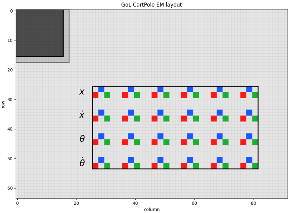
where
This EM is purely reactive and does not use state retention. At every CartPole macrostep, the board is reset to the same learned program
The learned program
The encoder
Each input bin (I) is paired with two nearby output-collector regions, one contributing to a left-force vote (L) and one contributing to a right-force (R) vote. The local motif is shown in Figure 12.
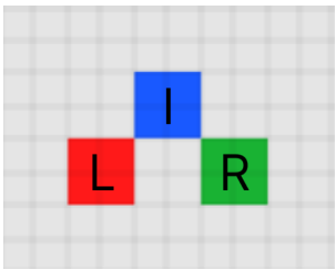
After encoding, the board evolves under the standard Conway’s GoL rule for a fixed computation time
i.e.
Then, the decoder aggregates activity over all left and right output-collector bins. Let
Where
Training uses a mutation-only genetic algorithm over gliders position, with occasional sparse binary mutation on the program region. For one episode, the fitness is
Importantly, the interface layout and computation time budget should be understood as simple heuristic design choices, not as the result of automated optimization over many possible interfaces. The budget
3.6.1 Results
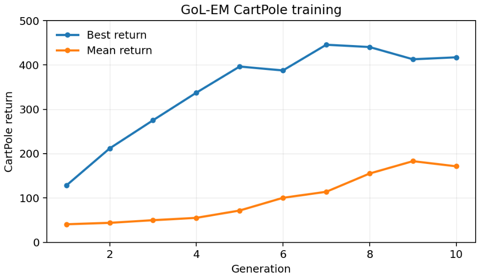
GoL-EM achieved CartPole returns clearly above the random baseline of
Qualitatively, the learned policy was simple but meaningful. The controller typically adopted a one-sided balancing strategy: it pushed the pole towards one side and then maintained balance through slow cart motion until eventually exiting the allowed position bounds. Since the vast majority of inspected episodes ended by exceeding the cart-position range rather than the pole-angle range, the policy appears to use angular information far more effectively than positional information, possibly ignoring positional information at all. This suggests that GoL-EM is capable of control behavior, but with several robustness-related limitations.
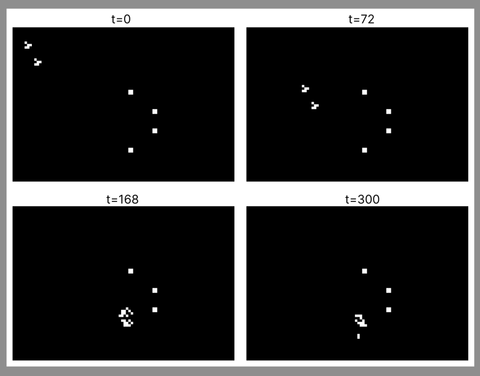
Figure 14 shows some representative snapshots of GoL state during a prediction. The dynamics are driven by glider motion and collisions with the encoded input blocks.
| Metric | Value |
|---|---|
| GoL computation budget | 300 |
| Population size | 100 |
| Training generations | 10 |
| Final population mean return | 171.36 |
| Best training return | 417.20 |
| Evaluation return | |
| non-halting rate | 54.5% |
We also briefly tested state retention by using the final GoL configuration from one CartPole macrostep to initialize the next (we employed identity retention
the present setting, this made the controller unstable and dropped its performance close to random, as residual debris from previous macrosteps accumulated and interfered with the next encoded observation in near-chaotic ways.
3.7 CEM1D
We then explored a continuous-valued, one-dimensional Emergent Model (CEM1D) for CartPole. This experiment differs from the previous GoL controller in two ways. First, the substrate is not a discrete binary cellular automaton, but a continuous-valued local dynamical system. Second, the controller uses retention across CartPole macrosteps: its internal state is retained from one control step to the next, rather than being reset after every action.
The latent state is a one-dimensional lattice of cells,
where
In our implementation, we integrate with explicit Euler steps of fixed size
Thus the model is implemented as a discrete dynamical system, although being motivated by a continuous-time update rule. Boundary conditions can be periodic, reflective, or zero-padded. In the representative run reported here, we used reflective boundaries.
We fix, once for all, a set of ports into the lattice as positions for writing/reading inputs and outputs. At each CartPole macrostep, the physical state
The system then evolves for a fixed duration of
After time evolution, a designated output cell
Equivalently,
The random tie-breaking region around zero is employed to avoid a degenerate control strategy observed in preliminary runs, where the controller exploited extremely small output values, for example on the order of
Only the local interaction parameters are explicitly trained. The latent state
As a representative minimally engineered configuration, we used a one-dimensional lattice of length

3.7.1 Results
In our experiments, the maximum episode length is 800 macrosteps. Fitness
where
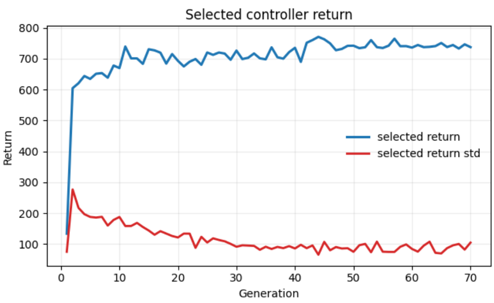
CEM1D learned high-performing CartPole policies, reaching returns close to the maximum of 800 and far above the random baseline of
reflects a real control policy rather than a lucky selection bias. (Results are summarized in Table 5 and the learning curves in Fig. 16).
| metric | value |
|---|---|
| generations | 70 |
| population size | 120 |
| lattice length | 19 |
| internal steps | 30 |
| input cells | |
| output cell | 9 |
| training return | |
| evaluation return |
Table 5: Results for a representative CEM1D CartPole training run.
For the selected controller, the learned update equation is:
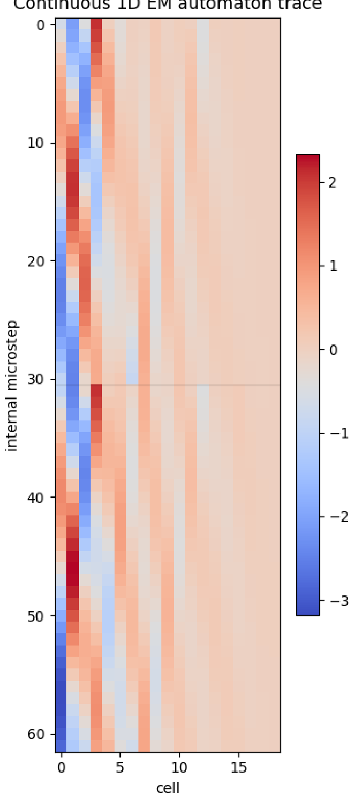
A representative space-time diagram of the automaton is reported in Fig. 17.
The learned policy substantially outperforms the GoL-EM controller and is very robust to deviations in the pole angle, but it still exhibits some fragilities. In nearly all manually inspected rollouts, the cart eventually drifted out of the allowed position range once enough time had passed. This occurred despite using a boundary-heavy initialization distribution, with 70% of training episodes starting near the cart-position boundaries to encourage robustness. Qualitatively, this suggests that the controller learned an effective pole-balancing strategy, but did not integrate correctly the cart-position information into its decision process.
This limitation is consistent with the structure of the
learned dynamics. The update rule is predominantly linear, and this may limit expressivity: the cubic term has a very small coefficient (0.03) and contributes substantially only when cell values become large, so for most of the operating range the lattice evolves close to a linear system. Two further design choices restrict expressivity: the fixed input and output port layout may constrain how the local dynamics can route information through the lattice, and the fixed computation time
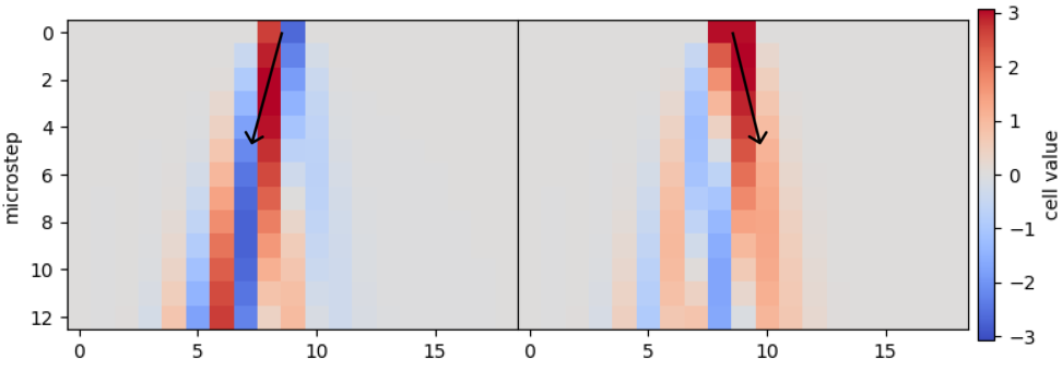
Interestingly, the evolved dynamics exhibit localized structures that behave like information carriers, similarly to gliders in discrete cellular automata (See fig. 18). In particular, two nearby cells with similar values tend to propagate their state to the right over successive microsteps, while two nearby cells with opposite values, forming a strong local gradient, tend to propagate information to the left. The left-moving transport appears stronger and more robust than the right-moving. This asymmetry may partly explain why position information, which would need to propagate rightward toward the output port, is used less effectively by the controller.
The CEM1D CartPole experiment should therefore be interpreted as an exploratory feasibility result rather than a mature control method. Nevertheless, the controller achieves high returns despite its limited use of cart-position information, comfortably exceeding the standard solution threshold of 500.
3.8 Meta-Life
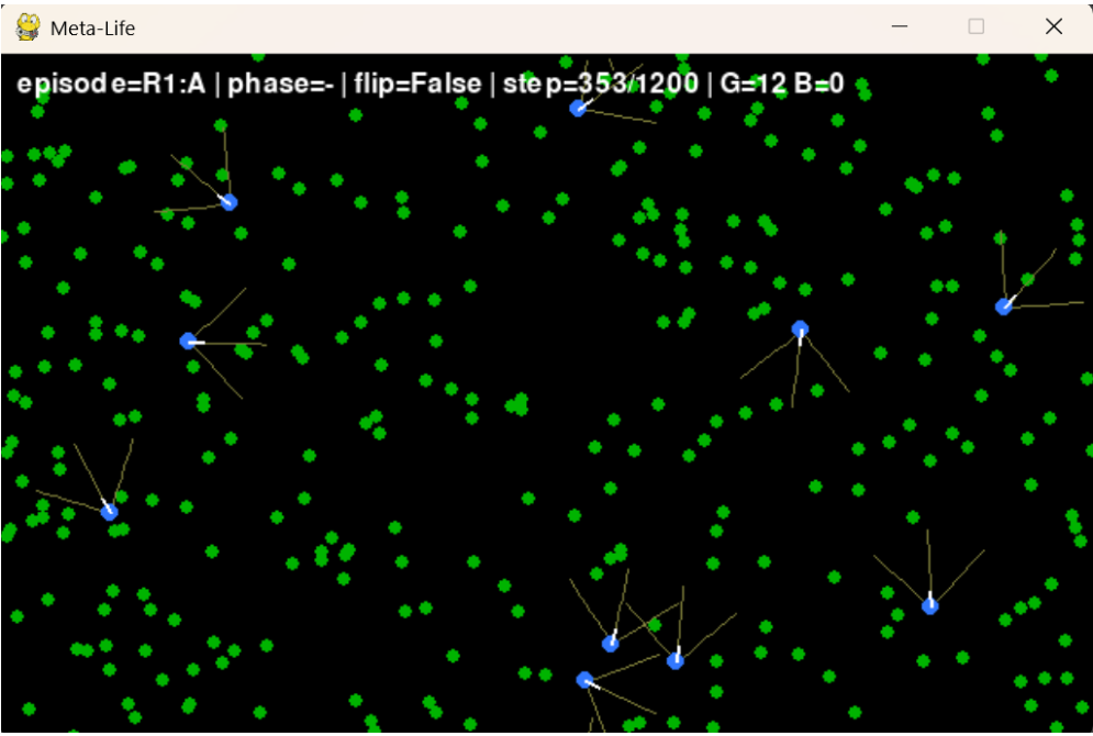
We next tested Emergent Models in a simple embodied environment, which we call Meta-Life. Meta-Life is a continuous two-dimensional toroidal world in which agents sense, navigate and collect resources (see fig. 19).
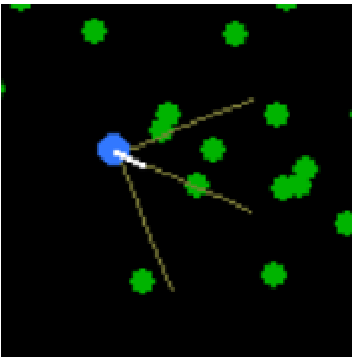
Each agent has a position in the 2D world and a heading that defines the direction it faces. It senses the environment through three lidar rays cast at fixed angles relative to its heading, so the rays rotate with the agent. Each ray returns a scalar in
The observation is therefore:
where
We consider two regimes. In Meta-Life-Food, every resource is food, and collecting one gives reward . This is an ordinary foraging task: the agent must use its lidar observations to steer toward food and collect it.
In Meta-Life-Adapt, resources alternate between food and poison in phases of random duration, while remaining visually identical: during a food phase, collecting any resource
gives reward
Each rollout consists of two mirrored episodes, A and B, each composed of four alternating phases. Episode A runs:
food (
and Episode B runs the same phases with reversed reward signs:
poison () food () poison () food ()
Here
We use two variance-reduction measures. First, the A/B symmetry above makes the score less sensitive to any particular phase-length sample, since each phase ordering is evaluated under both sign assignments. Second, each agent is evaluated over several rollouts per generation (
The observation is augmented with a transient reward-feedback signal:
where
For diagnostic purposes, we classify scores by their timing relative to the previous contact. A reward earned from a new contact within 6 macrosteps of the previous one falls in the reaction-window: the period in which the reward signal from that previous contact may still be present in the controller’s input. Rewards earned later fall in the after-reaction bucket.
After-reaction scores are therefore the stricter diagnostic: they measure whether the agent has inferred the current phase and retained it as a persistent internal memory, rather than merely reacting to the instantaneous reward signal. Since a phase lasts on average 300 macrosteps, far longer than the 6-macrostep reaction window, good adaptive behavior requires holding this phase memory across many reward-free macrosteps.
For a single agent and rollout, return is the cumulative reward:
where
For Meta-Life-Adapt, we also calculate the meta score:
A meta score of 0 indicates phase-insensitive behavior, i.e. no adaptation to the changing phases. A score of 1 indicates perfect selectivity, with only food contacts and no poison contacts, while a score of indicates the worst case, with only poison contacts and no food contacts. The term
During training, the food-only objective is the raw return reduced by two penalty terms:
where NaN or Inf appears in the action or in the model’s internal state.
Meta-Life-Adapt employs a slightly different objective:
The square root exponent forces diminishing returns in the absolute number of contacts. This reduces pressure to collect as many resources as possible and instead favors policies that are more selective, i.e. that maintain a good food/poison ratio even if collecting fewer total resources.
Meta-Life-Adapt tests in-distribution adaptation, a weaker regime than meta-learning: the agent must switch its policy online from the observed reward, but both regimes are seen during training and the model is never asked to adapt to a novel task. Online policy switching from a feedback signal is nonetheless a precondition for meta-learning, since a system unable to switch policy in response to reward could not adapt to unseen tasks. We therefore view this setting as a precursor to meta-learning.
CEM2D CEM2D is a continuous two-dimensional Emergent Model featuring a fully local update rule. Its state has two channels,
where
This state is paired with an interface
The encoder writes each observation component
where
We employ a fully local update rule
At each microstep, every cell first computes a scalar preactivation :
The activation field is then updated by a residual step:
The memory field is updated through a local write gate
The gate controls how strongly each memory cell moves toward the current activation at the same position: a closed gate leaves the memory unchanged, while an open gate moves it toward
All coefficients are global scalars, shared by all cells. The rates
After the
the decoder reads two output ports from the activation field and maps their values to the action
The retention operator used here is identity retention,
The fields and are retained not only across macrosteps but also across generations, using the Lamarckian-style state inheritance protocol described in Section 3: the selected parent’s final and fields are copied directly to its offspring, while crossover and mutation are applied only to the hard parameters.
Memory-augmented RNN baseline We compare CEM2D with a small dense memory-augmented recurrent neural network, denoted mRNN, featuring a fast hidden state
and decodes to:
Unlike CEM2D, this model uses dense recurrent matrices, so each hidden unit can depend on every hidden and memory component; its update rule is therefore nonlocal. Its state
| model | hard params size() | soft params size() | structure |
|---|---|---|---|
| CEM2D | 35 | 128 | local spatial fields |
| mRNN | 117 | 12 | dense vector recurrence |
As shown in Table 6, CEM2D employs relatively few hard parameters (fixed weights), while using a larger number of soft parameters (latent-state size). The mRNN has the opposite structure: it uses more hard parameters, but a smaller latent state. In CEM2D, the latent-state size is decoupled from the number of hard parameters, since the local update rule is shared across all cells and therefore independent of the lattice size. For the mRNN, by contrast, the two are coupled: the dense recurrent matrices make the number of hard parameters grow quadratically with the hidden-state dimension,
3.9 Training setup
Both controllers were trained with the same population-based genetic algorithm. At each generation, agents were evaluated over a fixed number of rollouts and were assigned a fitness score; the next generation was then produced through tournament selection, elitism, sparse crossover, and mutation. Under this scheme, an offspring inherited its hard parameters primarily from a base parent, with a donor parent contributing only a sparse subset of genes through crossover; these hard parameters were then mutated. Soft parameters, instead, were inherited unchanged from the base parent.
The food-only environment used population
| task | model | population | generations |
|---|---|---|---|
| Food-only | CEM2D | 100 | 700 |
| Food-only | mRNN | 100 | 700 |
| Meta-Life-Adapt | CEM2D | 300 | 510 |
| Meta-Life-Adapt | mRNN | 300 | 260 |
Table 7: Training setup for representative Meta-Life runs
3.10 Results
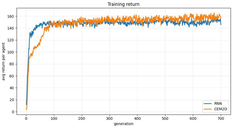
In Meta-Life-Food, both controllers learned effective food foraging policies. The mRNN learned faster early in training, while CEM2D caught up later and reached a comparable return. On evaluation, CEM2D reached a return of 133 per agent per rollout, while mRNN 146. (Results are shown in table 8, while learning curves in fig. 21).
| model | train return | eval return |
|---|---|---|
| CEM2D | 155 | 133 |
| mRNN | 150 | 146 |
Table 8: Meta-Life-Food results. Return is measured per agent per rollout.
Meta-Life-Adapt was more challenging: the mRNN achieved a meta-score about 15% higher than CEM2D. Nevertheless, both models obtained high meta-scores relative to the optimum value of 1, indicating successful adaptation in both cases. We also observed that CEM2D required substantially longer training and improved more slowly. (Results are shown in table 9).
| model | meta score | reaction meta | after-reaction meta |
|---|---|---|---|
| CEM2D | 0.714 | 0.780 | 0.699 |
| mRNN | 0.822 | 0.913 | 0.796 |
Table 9: Meta-Life-Adapt evaluation results. Random baseline is 0, perfect behaviour is 1.
Lamarckian inheritance of the
Two readings fit this: either is functionally useful, acting as a static “hardware” that shapes the computation; or is inert, and the collapse only reflects that the hard parameters co-adapted to the inherited state during training, so that ablating it moves them off the operating point they were fit to. A conclusive test would require two separate training runs:
one with the state inherited across rollouts and generations, as here, and one in which
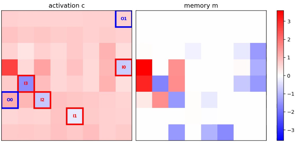
Interestingly, during inference we observe a phase-related interpretable feature near the reward input port
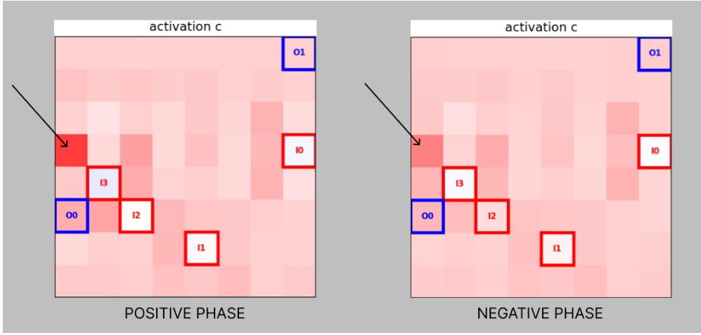
This cell also appears to modulate behavior. When its activation is high, the agent chases resources and collects them; when it is low, the agent rotates in place, reducing the chance of collecting poison. After the environment switches back to food, an eventual reward reactivates the cell, and the policy returns to resource-seeking. The resulting strategy is simple but effective: seek resources during food phases, rotate in place during poison phases. Although crude, it is sufficient to produce adaptation.
We observe several robustness-related failure modes, most visible on evaluation rollouts substantially longer than those seen during training. The most common is a rotating attractor, present in both CEM2D and in the mRNN: the agent rotates in place indefinitely, especially after a long period in which no resource enters its lidar rays. This occurs despite the looping penalty, though that penalty strongly mitigates it. The mRNN also exhibits a freezing failure: its learned policy permanently sets the velocity to zero after collecting poison, so the agent stops moving entirely and avoids further poison contacts in a risk-averse manner. Both failures share the same consequence: once the agent stops encountering resources, it can no longer taste one, update its regime estimate, or recover, and the policy remains stuck. In CEM2D this is compounded by spontaneous decay of the regime cell, whose activation gradually falls during long stretches without collecting food, pushing the policy toward persistent self-rotation.
Two aspects of the training setup plausibly explain these failures in both models. First, the fitness objective has diminishing returns: the square-root terms reward a high food/poison ratio rather than the raw number of foods collected, so a policy that gathers a few resources and then stops or rotates in place minimizes poison risk while sacrificing little of the expected fitness that further food collection would provide. Second, at each phase change all resources are removed and respawned at random locations. A respawned resource may enter the lidar rays of a rotating agent, or occasionally spawn on top of a frozen one. The agent is therefore rarely required to recover from a stuck state on its own.
4 Conclusion
In this work, we introduced Emergent Models as a framework for machine learning through simple, often local, iterated dynamical systems. Rather than treating modeling as the learning of a direct input-output map, EMs treat it as the search for configurations of a computational substrate whose time evolution gives rise to the desired behavior. The ingredients are minimal: a latent state space providing memory, an update rule allowing interactions within that space, an adaptive or sufficiently long computation time, and an interface connecting the substrate to external inputs and outputs.
Beyond abstracting ideas already present in Cellular Automata, Neural Cellular Automata, Neural GPUs, recurrent models, and classical computation theory, the formalism supports a broader position: computation relevant to learning need not reside in a prescribed abstract architecture, such as a neural network, but can emerge directly from a physical-like substrate and its initial conditions. The theoretical ground for this position is the Turing completeness of some simple dy-
namical systems, such as cellular automata. Classical universality, however, is attributed to the substrate alone: a cellular automaton is universal if some initial configuration simulates a universal Turing machine. Modeling asks for slightly more, namely a fixed, task-independent interface for writing inputs and reading outputs belonging to a general computable domain, such as binary strings
The experimental contribution is deliberately simpler, intended to validate the base idea of EMs as physical-like learning substrates, aiming to isolate first principles from the effects of scale, engineering, and architectural complexity. Whereas previous local-recursive modeling systems typically employ neural update functions with parameter counts on the order of
| model | substrate | hard params | soft params | param domain |
|---|---|---|---|---|
| EM43 | 1D CA | 60 | 10 - 50* | |
| GoL-EM (arith.) | 2D GoL | 0 | 100 - 300* | |
| GoL-EM (CP) | 2D GoL | 0 | 100 - 300* | |
| CEM1D | 1D CEM | 3 | 19 | |
| CEM2D | 2D CEM | 35 | 128 | mixed** |
| mRNN | dense RNN | 117 | 12 |
Table 10: Structural summary of the experimental models. * For EM43 and GoL, soft parameters are indicated as program region size. **For CEM2D: real-valued soft and update-rule parameters and integer-valued port locations.
| model | capabilities |
|---|---|
| EM43 | extrapolation on simple arithmetic tasks |
| GoL-EM (arithmetic) | limited capabilities on arithmetic tasks |
| GoL-EM (CartPole) | partially capable of control, not robust |
| CEM1D | stronger control capabilities, still not robust |
| CEM2D | capable of control and adaptation |
| mRNN | capable of control and adaptation, slightly stronger |
Table 11: Behavioral summary of the experimental models.
Among the individual results, the clearest is provided by EM43, which learns several simple integer functions and extrapolates perfectly far beyond the training range, including periodic functions that feed-forward neural networks cannot represent globally. In successful runs, generalization is not hidden in an opaque parameter vector: it appears as a stable space-time mechanism in the automaton’s diagram, a geometry of interaction that remains valid as the input scale increases. We refer to this phenomenon as geometric grokking, and it suggests that time- and translation-invariant substrates can host compact algorithmic routines whose structure is directly visible in their trajectories. Whether geometric grokking persists as task complexity increases, and whether it is partly an artifact of the particular tasks and interface choices employed, remains to be established.
Game of Life was difficult to exploit for learning. Its dynamics are highly sensitive to the initial condition: small changes in the program usually produce large, almost chaotic changes in behavior. This yields a brittle genotype-to-phenotype map and a weakly structured search space, in which similar programs have entirely different fitness, so the search has little local information to exploit and random sampling performs almost as well as evolutionary optimization. The difficulty is compounded by interface design: the interface adopted here, based on isolated
control tasks with real-valued inputs and outputs, they are more trainable and less brittle in their genotype-to-phenotype map, though still harder to train than feed-forward or standard recurrent models, which perform a single update per macrostep
The control experiments are further limited by the simplicity of the environments. CartPole is solvable by linear feedback controllers. In the non-adaptive Meta-Life setting, food attraction and poison avoidance may likewise be solvable by near-linear policies over the sensory inputs; even in adaptive Meta-Life, the required behavior may be achievable by near-linear policies operating on two time scales, fast action selection and slow phase memory, plus a nonlinearity acting as a fast switch that flips the phase memory on regime changes. More complex environments are therefore needed to evaluate the empirical advantages and limitations of Emergent Models relative to conventional neural controllers, especially in terms of generalization, adaptation, and robustness.
A single computational primitive ties the theoretical and empirical parts of this work together: iteration. We conjecture that applying a simple update rule for an adaptive number of steps is what lets a model extrapolate beyond a bounded input range, whereas a single forward pass only interpolates within it. This holds well beyond Emergent Models: adaptive-computation-time RNNs, reasoning transformers, and looped transformers
Among iterated systems, we conjecture that a further quantity governs the balance between generalization and trainability: the ratio of parametrization to temporal depth,
where
The preference for low
A second motivation is more speculative. The living world realizes adaptive, intelligent behavior even without nervous systems, through simpler physical and chemical mechanisms; and the nervous system itself is likely not fundamental, but a structure that physics supports: neurons obey physical laws and can be regarded as latent structures on top of a lower-level physics. Emergent Models operate at this more basic level, evolving a local rule and an initial configuration rather than a prescribed architecture. This does not exclude neural-network-like organization: if such a structure were the best solution for a task, it could in principle emerge within a latent-universal model. It does, however, reframe a question we cannot yet answer: whether the better route to intelligence on silicon is to build highly simplified models of biological neural networks, as artificial neural networks do, or to construct an artificial physics from which arbitrary structure can emerge. The Bitter Lesson would suggest the latter.
Two concrete directions follow. The first is to realize the latent-universal regime in practice, through a co-evolution of rules and programs under a fixed interface and halting operator. In a first phase, a rule shared across a distribution of tasks
is trained jointly with a separate program per task, and fitness selects for rules under which every task admits a solving program, pressuring toward a general rule. In a second phase, that rule is frozen and only the program is trained, on novel tasks of increasing complexity. Success would mean a fixed model that represents new functions by program changes alone. The second direction concerns scale, and bears directly on the trainability of low-
5 Acknowledgments
We thank the Wolfram Institute for research guidance, institutional affiliation, and support. We thank ResearchHub for supporting this project through an innovative decentralized science funding model. We are also grateful to everyone who contributed to this work through discussions, ideas, experiments, and encouragement. AI tools were used to assist with the implementation of the simulation code and language polishing of the manuscript. Outputs were verified for correctness and consistency. All scientific ideas, interpretations, and conclusions were developed by the authors.
References
- Emmanuel Abbe, Samy Bengio, Aryo Lotfi, Colin Sandon, and Omid Saremi. How far can transformers reason? the globality barrier and inductive scratchpad, 2024. arXiv.
- S. Arora and B. Barak. Computational Complexity: A Modern Approach. Cambridge University Press, 2009. ISBN 9781139477369. Google Books.
- J. Baxter. A model of inductive bias learning. Journal of Artificial Intelligence Research, 12:149–198, March 2000. ISSN 1076-9757. doi: 10.1613/jair.731. JAIR.
- Mark Braverman and Stephen Cook. Computing over the reals: Foundations for scientific computing, 2005. arXiv.
- Alexandra Butoi, Robin Chan, Ryan Cotterell, William Merrill, Franz Nowak, Clemente Pasti, Lena Strobl, and Anej Svete. Computational expressivity of neural language models. In Luis Chiruzzo, Hung-yi Lee, and Leonardo F. R. Ribeiro, editors, Proceedings of the 62nd Annual Meeting of the Association for Computational Linguistics (Volume 5: Tutorial Abstracts), pages 5–5, Bangkok, Thailand, August 2024. Association for Computational Linguistics. doi: 10.18653/v1/2024.acl-tutorials.3. ACL Anthology.
- François Chollet. On the measure of intelligence, 2019. arXiv.
- Matthew Cook. Universality in elementary cellular automata. Complex Systems, 15, 2004. Semantic Scholar.
- Emily Dolson, Sunny Kim, and Anya Vostinar. Open-ended evolution, 2024. ALife Encyclopedia. ALife Encyclopedia, International Society for Artificial Life.
- Benyamin Ghojogh and Ali Ghodsi. Recurrent neural networks and long short-term memory networks: Tutorial and survey, 2023. arXiv.
- Ian Goodfellow, Yoshua Bengio, and Aaron Courville. Deep Learning. MIT Press, 2016. Project website.
- Alex Graves. Adaptive computation time for recurrent neural networks, 2017. arXiv.
- Etienne Guichard. Critically pre-trained neural cellular automata as robot controllers. Master’s thesis, Delft University of Technology, April 2024. TU Delft. Cognitive Robotics, Faculty of Mechanical Engineering.
- Etienne Guichard, Felix Reimers, Mia Kvalsund, Mikkel Lepperød, and Stefano Nichele. Arc-nca: Towards developmental solutions to the abstraction and reasoning corpus, 2025. arXiv.
- Sumit Gulwani, Oleksandr Polozov, and Rishabh Singh. Program synthesis. Found. Trends Program. Lang., 4(1–2):1–119, July 2017. ISSN 2325-1107. doi: 10.1561/2500000010. DOI.
- Daya Guo, Dejian Yang, Haowei Zhang, et al. Deepseek-r1 incentivizes reasoning in llms through reinforcement learning. Nature, 645(8081):633–638, September 2025. ISSN 1476-4687. doi: 10.1038/s41586-025-09422-z. Nature.
- Ingo Gühring, Mones Raslan, and Gitta Kutyniok. Expressivity of deep neural networks, 2020. arXiv.
- Pamela J. Haley and Don Soloway. Extrapolation limitations of multilayer feedforward neural networks. [Proceedings 1992] IJCNN International Joint Conference on Neural Networks, 4:25–30 vol.4, 1992. Semantic Scholar.
- D. Harel and Y.A. Feldman. Algorithmics: The Spirit of Computing. Addison Wesley, 2004. ISBN 9780321117847. Google Books.
- Kurt Hornik. Approximation capabilities of multilayer feedforward networks. Neural Networks, 4:251–257, 1991. Semantic Scholar.
- Emil Jeřábek. Mathematical logic. Lecture notes, January 2026. Lecture notes, Charles University, Faculty of Mathematics and Physics. Based on course notes taken by Jindřich Novák. Accessed: 2026-06-15.
[21] Hongjian Jiang, Michael Hahn, Georg Zetzsche, and Anthony Widjaja Lin. Softmax transformers are turing-complete, 2025. URL arXiv.
[22] Alexia Jolicoeur-Martineau. Less is more: Recursive reasoning with tiny networks, 2025. URL arXiv.
[23] J.R. Koza. Genetic Programming: On the Programming of Computers by Means of Natural Selection. A Bradford book. Bradford, 1992. ISBN 9780262111706. URL Google Books.
[24] Sreejan Kumar, Ishita Dasgupta, Nathaniel D. Daw, Jonathan D. Cohen, and Thomas L. Griffiths. Disentangling abstraction from statistical pattern matching in human and machine learning, 2023. URL arXiv.
[25] Gary Marcus. Deep learning: A critical appraisal, 2018. URL arXiv.
[26] Arnold W. Miller. Lecture notes in computability theory. Project website, December 2008. Lecture notes for Math 773, Fall 2007, University of Wisconsin–Madison.
[27] Alexander Mordvintsev, Ettore Randazzo, Eyvind Niklasson, and Michael Levin. Growing neural cellular automata. Distill, 2020. doi: 10.23915/distill.00023. Distill.
[28] Stefano Nichele and Andreas Molund. Deep reservoir computing using cellular automata, 2017. URL arXiv.
[29] Nicolas Ollinger. Universalities in cellular automata; a (short) survey. In Bruno Durand, editor, Proceedings of the First Symposium on Cellular Automata ”Journées Automates Cellulaires”, Regular paper track, pages 102–118, Uzès, France, April 2008. Izdatel’stvo MTsNMO. URL hal.science. ISBN 978-5-94057-377-7.
[30] OpenAI. Learning to reason with LLMs. OpenAI, September 2024. Accessed: 2026-03-18.
[31] Alec Radford and Karthik Narasimhan. Improving language understanding by generative pre-training, 2018. URL Semantic Scholar.
[32] Paul Rendell. Turing Machine Universality of the Game of Life, volume 18 of Emergence, Complexity and Computation. Springer International Publishing, 1 edition, 2016. ISBN 978-3-319-19842-2. doi: 10.1007/978-3-319-19842-2.
[33] Parshin Shojaee, Iman Mirzadeh, Keivan Alizadeh, Maxwell Horton, Samy Bengio, and Mehrdad Farajtabar. The illusion of thinking: Understanding the strengths and limitations of reasoning models via the lens of problem complexity, 2025. URL arXiv.
[34] M. Sipser. Introduction to the Theory of Computation. Cengage Learning, 2012. ISBN 9781133187790. URL Google Books.
[35] Laura Strieker. On the progression of finding the smallest known universal Turing machine, 2020. URL thi.uni-hannover.de. Fakultät für Elektrotechnik und Informatik, Institut für Theoretische Informatik.
[36] Richard S. Sutton. The bitter lesson. Incomplete Ideas (blog), March 2019. incompleteideas.net, accessed 2026-06-15.
[37] R.S. Sutton and A.G. Barto. Reinforcement Learning, second edition: An Introduction. Adaptive Computation and Machine Learning series. MIT Press, 2018. ISBN 9780262352703. URL Google Books.
[38] Teun D.H. van Nuland. Noncompact uniform universal approximation. Neural Networks, 173:106181, May 2024. ISSN 0893-6080. doi: 10.1016/j.neunet.2024.106181. URL ScienceDirect.
[39] Joaquin Vanschoren. Meta-learning: A survey, 2018. URL arXiv.
[40] Alexandre Variengien, Stefano Nichele, Tom Glover, and Sidney Pontes-Filho. Towards self-organized control: Using neural cellular automata to robustly control a cart-pole agent, 2021. URL arXiv.
[41] Guan Wang, Jin Li, Yuhao Sun, Xing Chen, Changling Liu, Yue Wu, Meng Lu, Sen Song, and Yasin Abbasi Yadkori. Hierarchical reasoning model, 2025. URL arXiv.
[42] K. Weihrauch. Computable Analysis: An Introduction. Texts in Theoretical Computer Science. An EATCS Series. Springer Berlin Heidelberg, 2000. ISBN 9783540668176. URL Google Books.
[43] L. D. Whitley. A genetic algorithm tutorial. Statistics and Computing, 4:65–85, 1994. URL Semantic Scholar.
[44] Wikipedia contributors. Expressive power (computer science). Wikipedia, 2026. [Online; accessed 15-June-2026].
[45] S. Wolfram. A New Kind of Science. Wolfram Media, 2002. ISBN 9781579550080. URL Google Books.
[46] Stephen Wolfram. What is ChatGPT doing … and why does it work? Stephen Wolfram Writings, February 2023. URL stephenwolfram.com. Accessed: 2026-06-15.
[47] Kevin Xu and Risto Miikkulainen. Neural cellular automata for arc-agi, 2025. URL arXiv.
[48] Ozgur Yilmaz. Reservoir computing using cellular automata, 2014. URL arXiv.
[49] Rui-Jie Zhu, Zixuan Wang, Kai Hua, Tianyu Zhang, Ziniu Li, Haoran Que, Boyi Wei, Zixin Wen, Fan Yin, He Xing, Lu Li, Jiajun Shi, Kaijing Ma, Shanda Li, Taylor Kergan, Andrew Smith, Xingwei Qu, Mude Hui, Bohong Wu, Qiyang Min, Hongzhi Huang, Xun Zhou, Wei Ye, Jiaheng Liu, Jian Yang, Yunfeng Shi, Chenghua Lin, Enduo Zhao, Tianle Cai, Ge Zhang, Wenhao Huang, Yoshua Bengio, and Jason
Appendix
A.1 Turing machines as Emergent Models
Turing Machines can be represented as generalized automata (see Figure 24 for a graphical representation).
Let
The global alphabet is
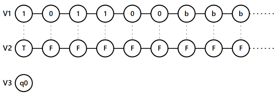
The halting predicate reads the control vertex and returns 1 exactly when
A.2 Universal Turing machines
A universal Turing machine
If the combining operator
We are, however, particularly interested in constructions that admit a disjoint formulation: program and encoded input occupy separate regions, or separate tapes,
A.3 Proof sketch of Theorem 1
Let
Fix a strongly universal Turing machine
For the target function
Finally,
Lemma 2 (GoL admits latent universality). There exists an Emergent Model
Sketch. Treat GoL as a generalized automaton with state space
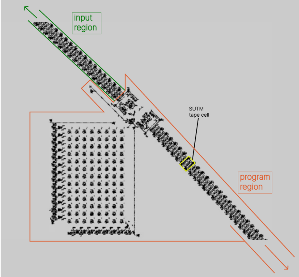
A.4 Computation and Modeling on the Continuous
In the main text, we define exact computation for discrete functions and arbitrary-precision approximation for continuous-valued functions. Here we make the latter notion more explicit.
Standard computable analysis usually treats real numbers through infinite representations (a real input may be represented by an infinite name). A machine can then read as much of this infinite representation as needed to produce an output to a requested accuracy.
We use a different (and simpler) formulation: inputs are discretized to arbitrary precision and encoded as finite strings. This keeps the framework close to ordinary computation theory.
A.4.1 Finite dyadic representations
Let
be the set of dyadic rationals. These are numbers with finite binary representations, and can therefore be encoded as finite strings.
The set
Equivalently, by increasing the number of binary digits, the dyadic grid becomes finer, and finite dyadic numbers can approximate any real number arbitrarily closely.
Thus, the model receives a finite dyadic approximation of the input,
A.4.2 Exact computation on dyadic inputs
On dyadic inputs, computation is ordinary discrete computation. A model
Let:
be a dyadic-valued partial computable function, total computable on the subset
and
A universal Turing machine operating on finite dyadic representations can compute exactly any partial computable dyadic function, halting on inputs in the domain and diverging otherwise.
A.4.3 Continuous computation as arbitrary-precision approximation
Now let:
be a continuous-valued partial function, total in the domain
In this setting, we use the word computes in the arbitrary-precision approximation sense, as input and output are finite precision dyadic representations.
For every output tolerance
The output tolerance
A.4.4 Asymptotic form
The same idea can be written asymptotically in terms of input precision. We consider the case where, for every real input
Fix an output tolerance
The model computes if, for every
Equivalently,
Thus, for each requested output tolerance
A stronger theoretical question, not addressed here, is whether as
Footnotes
-
Expressivity concerns whether a target function lies in the representable class at all (an existence question), while inductive bias concerns which representable solution training tends to select from finite data. The two are related: a model can only be biased toward a solution that it is first able to express, so expressivity is a precondition for inductive bias. ↩
-
For example, periodic activations or Fourier features for . ↩
-
Three notions of universality are most commonly distinguished for CAs. Weak universality employs an infinite periodic pattern, Strong universality requires an infinite quiescent background, Intrinsic universality is stronger still: can simulate any other CA under a fixed block rescaling of space and time. [29]. ↩ -
GA hyperparameters varied slightly by task. Typical ranges were: program mutation rate 0.02–0.06; rule mutation rate 0.01–0.04; program crossover rate 0.03–0.07; rule crossover rate 0.02–0.06; density penalty ; invalid-run penalty 5; tournament size 2; elite fraction 0.05; random-immigrant fraction 0.05; cross-island immigrant fraction 0.01; cross-island migration every 10–30 generations. ↩ -
Given that weak universality already appears in the 2-state, radius-1 case through Rule 110. ↩