ScholarOne Manuscripts

Growing Echo State Networks through Graph-Based Morphogenesis with Developmental Graph Cellular Automata

Matias Barandiaran${}^1$, James Stovold${}^2$

Corresponding: James Stovold (james.stovold@york.ac.uk)

${}^1$ Lancaster University Leipzig, Nikolaistraße 10, 04109 Leipzig, Germany
${}^2$ Department of Computer Science, University of York, York, YO10 5DD, United Kingdom

Abstract. Developmental Graph Cellular Automata (DGCA)D G C A are a novel model of morphogenesis, capable of growing directed graphs from single-node seeds. In this paper, we extend the DGCA model to exhibit stochastic growth, and show that both deterministic and stochastic DGCAs can be trained to grow reservoirs. Reservoirs are grown with two types of targets: task-driven (using the NARMA family of tasks) and task-independent (using reservoir metrics).

Results show that deterministic DGCAs are able to grow a variety of specialised, life-like structures capable of solving benchmark tasks, outperforming ‘typical’ reservoirs on the same task. Stochastic DGCAs grow robust, regular structures that outperform reservoirs grown deterministically. Overall, these lay the foundation for the development of DGCA systems that produce plastic reservoirs and for modelling functional, adaptive morphogenesis.

Keywords: Reservoir Computing, Cellular Automata, Stochastic Growth, Developmental Computing, Graph Growth, Morphogenesis

1 Introduction

Morphogenesis orchestrates the development of complex life. Through morphogenesis, populations of cells collaborate to form intricate structures such as eyes, limbs, and hearts. This process arises entirely from local interactions. Despite cells acting only on information from their immediate neighbourhood, the collective outcome is globally coherent. This capacity for self-organisation, where complex order emerges from decentralised rules, has long fascinated the scientific community (Turing, 1952).

Mordvintsev et al. (2020)Mordvintsev and colleagues introduced Neural Cellular Automata (NCA) as a computational model of morphogenesis. By leveraging neural networks as the transition rule of a cellular automaton, NCAs can learn to grow predefined two-dimensional shapes from a single-cell seed. An important property of this approach is its robustness: grown structures can re-generate their target shape after perturbation, with recent efforts reducing NCA instability by introducing an identity layer (Stovold, 2025). NCAs, however, lack an important biological nuance: in nature, structures do not emerge solely for their shape but to serve a purpose. In this study, that purpose is computation.

Developmental Graph Cellular Automata (DGCA) (Waldegrave et al., 2023)introduced by Waldegrave and colleagues extend NCAs by enabling the growth of directed graphs. Rather than growing shapes on a fixed grid, DGCAs allow a graph to grow from a single-node seed through a distributed process. Directed graphs are particularly well suited for representing recurrent neural networks (RNNs), which excel at modelling sequential data and have become powerful tools in tasks such as time series prediction and natural language processing (Mienye et al., 2024). This makes DGCAs a natural candidate for exploring the growth towards a functional target.

Despite their utility, training RNNs is computationally intensive due to their reliance on backpropagation through time. RNNs also suffer from the well-known problem of vanishing and exploding gradients, leading to numerical instability and a limited ability to capture long-range temporal dependencies (Bengio et al., 1994). Reservoir Computing (RC) was

developed as a response to these challenges (Lukoševičius & Jaeger, 2009)Lukoševičius and Jaeger, 2009. In the RC framework, an Echo State Network (ESN)E S N consists of a large, fixed, randomly connected RNN—known as the reservoir—which provides rich nonlinear dynamics while only the read-out layer is trained to solve a task.

A key appeal of RC is its ability to leverage physical reservoirs. This scheme’s flexibility allows for a wide range of dynamical systems exhibiting the echo state property to serve as successful reservoirs (Nakajima, 2020)Nakajima, 2020; including cultured biological neurons (Sumi et al., 2023)Sumi and colleagues, 2023, nanomaterial probes (Qi et al., 2023)Qi and colleagues, 2023, or even an octopus arm replica (Nakajima et al., 2013)Nakajima and colleagues, 2013. Attention toward Physical Reservoir Computing (PRC) over conventional von Neumann architectures reflects a shift to exploiting the intrinsic dynamics of physical systems. PRC opens a route to low-power computation, continuous signal processing, and robust fault tolerance in ways that traditional architectures struggle to achieve (Yan et al., 2024)Yan and colleagues, 2024.

Conventional RC relies on brute-force methods, i.e. randomly initialising multiple reservoirs in turn until the appropriate dynamics are found. The search is often done randomly or by novelty-based methods. While some work has applied optimisation algorithms (Soltani et al., 2023)Soltani and colleagues, 2023, they often serve only to refine this brute-force approach. In PRC, the challenge is even greater: physical substrates are often selected based on general computational potential (Dale et al., 2019)Dale and colleagues, 2019, with little opportunity to actively design or adapt the system.

This raises a fundamental question: why not use DGCAs to grow our own reservoirs? Previous applications of DGCAs have focused on growing graphs with specific structural features, such as motif distributions (Waldegrave et al., 2024)Waldegrave and colleagues, 2024. In this work, we grow directed graphs based on task performance as well as task-independent metrics, laying the foundation for DGCA systems capable of producing plastic reservoirs. Plastic reservoirs can adapt to changes in the environment or task and recover functionality after sustaining damage. We also find that specialisation emerges naturally through task-driven growth. Instead of

relying on a “one-size-fits-all” reservoir, we can grow reservoirs that prioritise certain RC metrics without explicitly optimising for them.

To better reflect the principles of biological development, we revisit a property that many computational models overlook. Development in natural systems is not deterministic; stochastic fluctuations in local interactions can facilitate organised pattern formation (Galbraith et al., 2022)as shown by Galbraith and colleagues in 2022. We incorporate controlled randomness into the sensing mechanism of DGCA cells. Rather than destabilising growth, stochasticity enhances robustness and, in several cases, yields reservoirs that outperform deterministic counterparts.

Beyond growth dynamics, the role of topology in RC has received little attention. Reservoirs are usually treated as complex, nonlinear black boxes. Aven et al. (2024)Aven and colleagues attempted to peek into this black box by shrinking and growing lattice reservoirs, revealing salient features. In this work, we find that certain topologies tend to emerge for specific tasks; we systematically classify these for downstream analysis. While random initialisation often leads to small-world reservoirs, most structures we observe are sparse and “life-like”. Together, these findings bring us closer to a functional and adaptive model of morphogenesis.

2 Developmental Graph Cellular Automata

Conventional Cellular Automata (CA) consist of a grid of cells, each of which can be dead or alive. Neural Cellular Automata (NCA) (Mordvintsev et al., 2020)by Mordvintsev and colleagues extend the CA framework by replacing the rule-based update mechanism with a neural network trained to evolve the cell states so that a desired overall pattern emerges from an initial single-cell seed.

Biology, however, does not work on a grid, as cells have an irregular number of neighbours. To better capture the complexity of biological environments, Graph Cellular Automata (GCA) (Marr & Hütt, 2009)proposed by Marr and Hütt generalise the traditional CA framework by organising cells in a graph structure, where nodes represent cells and edges represent connections

Figure 1: DGCA pipeline of a two-state (black and white) system. The neighborhood information vector $\mathbf{G}$G is shown for node $\mathbf{X}$X. The action Multi-Layer Perceptron (MLP) determines that $\mathbf{X}$X and $\mathbf{Y}$Y divide, while $\mathbf{Z}$Z is removed. $\mathbf{G}$G is gathered a second time, now with zero incoming black node connections but an additional white one, before being passed to the state Single-Layer Perceptron (SLP). Adapted from Figure 4 of (Waldegrave et al., 2024)Figure 4 of Waldegrave and colleagues, 2024.

between them. Despite providing a more flexible environment, efforts put into learning GCAs (Grattarola et al., 2021)Grattarola and colleagues have focused on self-organisation rather than growth (i.e.,that is, geometric point cloud reconstruction with a fixed number of nodes).

Najarro et al. (2023)Najarro and colleagues developed Neural Developmental Programs to grow artificial neural networks from seed graphs. Although this approach operates locally in an architectural sense, it is not strictly local in its information horizon. Before any growth decision is made, node states are propagated via graph convolutions for a number of steps equal to the network diameter, allowing each node to aggregate distant information. More importantly, the graphs they produce are undirected, making them less suitable for representing RNNs.

Waldegrave et al. (2023)Waldegrave and colleagues introduced Developmental Graph Cellular Automata (DGCA) as an extension to NCAs, GCAs, and L-Systems (Lindenmayer, 1968)Lindenmayer, 1968. DGCAs allow for a graph to start from a single node and expand over time. Using information about their own and immediate neighbouring states, nodes can decide when to divide, controlling the growth process in a distributed way. This work builds upon the more recent variant, DGCA-M (Waldegrave et al., 2024)Waldegrave and colleagues, 2024, which splits the update step into two stages: action and state.

Figure 2: Possible edge choices for a newly created node $X^{\prime }$X prime resulting from division of $X$X. Adapted from Figure 6 of (Waldegrave et al., 2024)Waldegrave and colleagues, twenty twenty-four.

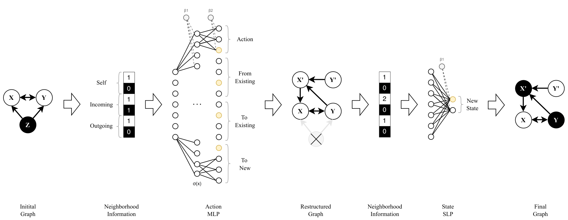
For each node in a particular graph, the DGCA follows the steps below (visualised in Figure 1) at each timestep to determine how the graph should change.

1. A neighbourhood aggregation function is used to build a vector for each node, capturing its own state and its local connectivity. The vector concatenates the node’s one-hot state with two state count histograms (incoming and outgoing neighbours). Figure 1 shows this neighbourhood information vector for node $X$X.

2. The resulting neighbourhood vector is passed to a small neural network (the action Multi-Layer Perceptron (MLP)), which determines each node’s behaviour: removal, division, or stasis. All decisions are made at the level of individual nodes, based exclusively on local information. The MLP output has dimension 15, split into four sections. The first section contains three values (one per action), and the action is selected via the argmax function. If removal or stasis is chosen, the remaining 12 values are ignored. If division is chosen, the remaining values are split into three groups of four (with argmax applied in each group).

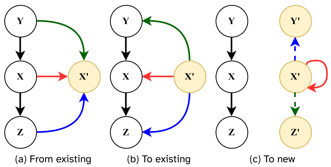
3. The MLP output is used to restructure the graph according to the valid edge choices for newly created nodes shown in Figure 2. These are grouped into three categories: From Existing, To Existing, and To New. In order to prevent the graph from becoming

overly dense, nodes are allowed to select one set of edges (blue, red, green) from within each category. Each category corresponds to one of the three remaining sections of the MLP output. Within each section, three values map to one of the edge sets, while the fourth value represents None.

4. Once the graph topology is updated, each node’s neighbourhood vector is recomputed.

5. The updated vectors are passed through another small neural network, the state single-layer perceptron (SLP), which determines the new internal states of the nodes for the next timestep. Figure 3 shows how these states help orchestrate growth.

For further detail about the DGCA-M and how it operates on graphs, the reader is directed to (Waldegrave et al., 2024)Waldegrave and colleagues, 2024.

3 Methods

We extend the DGCA-M model to better suit reservoir growth. As many of the rules in conventional Cellular Automata (CA) are not linearly separable (Minsky & Papert, 1969)as shown by Minsky and Papert, we replaced the ‘action’ Single-Layer Perceptron (SLP) with a 2-layer Multi-Layer Perceptron (MLP) with 64 nodes in the hidden layer (see Figure 1). Additionally, nodes that emerge with a degree of zero (isolated) are dropped.

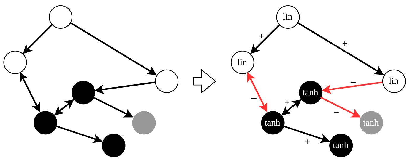
The original DGCA framework produces graphs with binary weights. We bipolarise the graphs to enable more complex dynamics, with edge weights assigned values of either $+1$plus one or $-1$minus one. Each weight is determined by the direction of the edge and the states of the connected nodes. By restricting weights to a discrete bipolar scheme, we decouple topology from weight tuning, pushing the DGCA to grow effective structures without optimising continuous weight values. Node states are also mapped to activation functions (e.g. tanh, linear), allowing for multiple types of neuron behaviour. We showcase the bipolarisation

Figure 3: Non-monotonic growth of a single graph (steps 8-19), read left to right and top to bottom. Node colour encodes cell state (red/blue); only red cells divide. At steps 9-10, 11-12, 13-14, 15-16, and 17-18, node count stays fixed while only leaf-node states toggle. The graph then resumes growing, with node count increasing at the following step. This alternation between state-only updates and division shows how a cell’s decision depends on its own and its neighbours’ current state.

step of a simple system in Figure 4. This study uses a three-state system: one linear and two tanh states. Mapping two states to tanh allows both positive and negative weighted interactions between nodes in those states.

We also extended the model’s sensing phase (neighbourhood information, see Figure 1) with an option for stochasticity, introduced by perturbing the cells’ observed local connectivity. Noise is interpreted as an exploration rate $\eta \in [0,1]$eta between zero and one that probabilistically alters the perceived neighbourhood of each node. Existing edges may be removed with probability proportional to $\eta$eta, while new connections may be introduced with probability scaled by

Figure 4: Bipolarisation step of a three-state system. Weights between differing states are negative ($-1$). Weights between equal states are positive ($+1$). White state nodes represent linear neurons, while black and blue state nodes represent tanh neurons. By including two separate states for tanh, we allow for both positive and negative weights between tanh neurons.

Table 1: Summary of hyperparameter configuration.

both $\eta$eta and the current graph density. For an adjacency matrix $A$A, the perturbed matrix $\tilde{A}$A tilde is defined element-wise as

where ${\mathcal{U}}_{ij}\sim \text{Uniform}(0,1)$U i j is sampled from a uniform distribution between zero and one and $\rho (A)$rho of A is the graph density. This scaling preserves the overall magnitude of connectivity while allowing for controlled structural variation.

To search for DGCA genotypes capable of producing well-performing reservoirs across multiple growth instances in stochastic experiments, we grow 5 reservoirs per chromosome pair per trial, assigning each contestant a fitness score equal to the average performance across all 5 reservoirs. Find a summary of all hyperparameters in Table 1.

3.1 Search

Since the DGCA update function is non-differentiable, algorithms like backpropagation are not viable for the search. Instead, we use a variant of the classic Microbial Genetic Algorithm (MGA) (Harvey, 2011)proposed by Harvey in 2011 to find the weights. This variant extends the standard MGA by introducing a double chromosome encoding. A chromosome is a flattened vector of weights and biases belonging to either the action MLP or the state SLP. An individual’s genotype is the pairing of one MLP chromosome with one SLP chromosome which together form a DGCA instance. The genotype specifies the update rule used to grow a reservoir. That grown reservoir is the phenotype, the structure evaluated and assigned a fitness score. Selection acts on the phenotype, while inheritance and mutation act on the genotype.

We initialise a population of 10 chromosomes per neural network type (action and state), resulting in 100 “genetically complete” individuals. To preserve internal dependencies and

minimise fragmentation risk, the MLP is encoded as a single chromosome rather than split by layer. Crossover, however, respects layer boundaries so weights belonging to layer $i$i of the winner can only replace weights belonging to layer $i$i of the loser. Each iteration of the MGA proceeds as follows:

1. Two DGCA individuals are selected at random from the population to compete. Due to stochastic selection, not all possible individuals are guaranteed to be evaluated in a given run.
2. For each DGCA, a reservoir is grown, evaluated, and assigned a fitness score based on the chosen fitness function.
3. The lower-scoring individual (loser) receives 50% of the higher-scoring individual’s (winner’s) genetic material. This transfer is performed independently for each chromosome type: MLP weights are only exchanged with MLP weights, and SLP weights only with SLP weights.
4. The loser undergoes a 2% mutation rate, introducing random perturbations to its weights.

3.2 Experimental Design

Each experiment consists of 150 runs, where each run involves 1000 iterations of the MGA. Within each iteration (trial) two reservoirs compete against each other. This results in a total of at least $150\times 1000\times 2=300,000$one hundred fifty times one thousand times two, which equals three hundred thousand reservoir instances (not necessarily unique) generated per experiment. To grow each reservoir, the DGCA update pipeline is executed 100 times, starting from a single node seed. DGCAs are given a node budget integrated into the MGA logic: if a grown reservoir exceeds the permitted size, it is assigned a fitness score of 0.

We conducted two broad types of experiments: task-driven and task-independent. In task-

driven experiments, reservoirs are grown and evaluated directly against a benchmark task, while in task-independent experiments, reservoirs are evaluated against established RC metrics as proxies for general computational capacity.

To calculate the fitness on the task-driven experiments, approximately two-thirds of the reservoir is perturbed with the input signal. Reservoir topology remains fixed throughout training and evaluation, consistent with the traditional RC framework. Input weights are randomly generated from the discrete set $\{-1,0,+1\}$minus one, zero, plus one, assigning each value with equal probability. In this work, we keep the fraction of input nodes static, but this could be easily varied in future. Similarly, we keep the input gain and feedback gain static at 0.1 and 0.95, respectively. The input gain scales the strength of the signal entering the reservoir, and the feedback gain controls the influence of the previous output fed back into the reservoir. For further details on reservoir computing, the reader is guided to (Lukoševičius, 2012)Lukoševičius, twenty twelve.

Once the reservoir state is computed, the readout layer is trained using Bayesian ridge regression between the state and target output. The regression is run for 3000 epochs, with a learning rate of $1e-6$one e to the minus six. The reservoir’s performance is evaluated using the normalised mean square error (NMSE) between the true and predicted sequences.

To mitigate variance caused by randomly initialised input weights, we perform 5 measurements. This is different from the 5 reservoirs measured in stochastic experiments, resulting in 25 measurements per individual per MGA trial in the stochastic experiments. The model is also compared to a control case: randomly initialised reservoirs under similar constraints (bipolar weights and comparable density)—i.e., ‘normal’ Echo State Networks (ESNs).

We chose the NARMA (Normalised Auto-Regressive Moving Average) family of tasks to drive the optimisation. NARMA tasks are widely used as benchmarks for the imitation of open systems. These are dynamical systems whose current output depends not only on the current input but on a history of past inputs and outputs. We will be using the

Figure 5: 50 timesteps of the NARMA-10, -20, and -30 target output sequences generated from the same input signal.

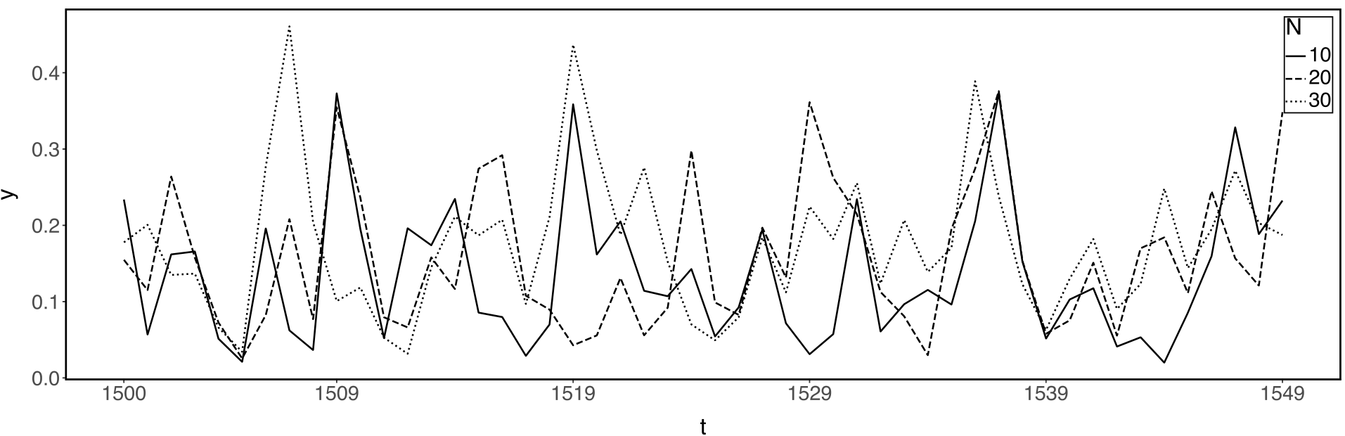
generalised $N$-th orderN-th order, referred to as NARMA-$N$NARMA N (Rodan & Tiňo, 2010)by Rodan and Tiňo. As $N$N increases, the reservoir must effectively retain and process a longer history of states to compute the output, making the task more challenging. A sample of 50 timesteps for $N=10,N=20$N equals 10, N equals 20, and $N=30$and N equals 30 is shown in Figure 5, showcasing the output’s nonlinearity; all three orders are used in our experiments. Following the implementation provided in (Trouvain et al., 2020)by Trouvain and colleagues, the system evolves according to:

In this study, the input signal $u(t)$u of t is independently drawn from a uniform distribution over the interval $[0,0.5]$zero to zero point five. The full $u(t)$u of t is fed into the reservoir before the readout is trained, as described above. The parameters are set to

In contrast, the task-independent experiments evaluated reservoirs using four widely-accepted RC metrics, as summarised in (Wringe et al., 2024)by Wringe and colleagues: Kernel Rank (KR), Generalisation Rank (GR), Linear Memory Capacity (LMC), and Spectral Radius (SR). Rather than measuring

performance on specific tasks, these metrics capture computational properties intrinsic to the reservoir. KR reflects the reservoir’s ability to separate dissimilar inputs (Legenstein & Maass, 2007)as described by Legenstein and Maass; GR quantifies robustness to noise by measuring generalisation over similar inputs (Legenstein & Maass, 2007)also by Legenstein and Maass; LMC quantifies fading memory (Jaeger, 2001b)as shown by Jaeger; and SR is often associated with a reservoir’s operation near the edge of chaos (Jaeger, 2001a)also discussed by Jaeger. We use these metrics as fitness functions: for KR, GR, and LMC, higher values indicate greater fitness; for SR, fitness is measured by proximity to 1, with lower distance being better. We also incorporate all four of these metrics into a single aggregate (All).

Figure 6: Distribution of task performace (higher is better) for NARMA-10 grown reservoirs across node budgets. Pairwise comparisons used independent two-sample U-tests with Bonferroni correction ($\alpha =0.05$alpha equals zero point zero five, corrected threshold $p<0.0167$p less than zero point zero one six seven). Significant differences: 100 vs 200 ($p=6.215e-20$), Control vs 200 ($p=1.852e-23$), Control vs 100 ($p=2.830e-15$).

4 Results

This section presents an analysis of the grown reservoirs and demonstrates how their performance varies based on budget and fitness functions. For each MGA run (i.e. 1000 iterations), the best-performing reservoir is selected based on the fitness function, resulting in 150 fittest reservoirs per experiment.

4.1 Task-Driven Growth: NARMA-10

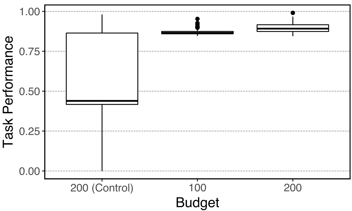
In this section, we aimed to evaluate how the model compares to randomly initialised Echo State Networks (our control case), under varying budget allocations for NARMA-10 growth. Here, Budget refers to the maximum number of permitted neurons in the reservoir.

Figure 6 shows the task performance (inverse NMSE; higher is better) on NARMA-10 for the fittest reservoirs in three settings: 200 (Control), 100, and 200 node budgets. Growing the reservoir for the task consistently outperforms random initialisation, even when the

Figure 7: Budget usage (%) distribution of NARMA-10 grown reservoirs across node budgets.

Table 2: Task-independent properties of NARMA-10 grown reservoirs. Values are reported as median (interquartile range). Each row corresponds to an experiment, while each column corresponds to a metric computed from the fittest reservoirs. Kernel Rank (KR), Generalisation Rank (GR), and Linear Memory Capacity (LMC) are normalised by the number of nodes.

grown reservoirs have only half the neurons of the control. As expected, increasing the budget leads to improved performance, with a significant increase observed between 100 and 200 nodes.

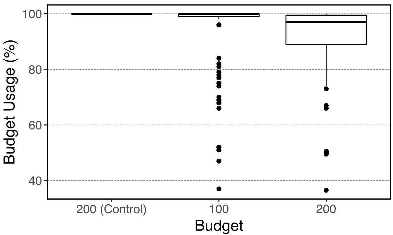
Despite being given a budget, the DGCA model is not required to use all of it. Figure 7 shows that many reservoirs did not use the full neuron budget, with some using less than 40% (even in the 100-node experiment). Relative budget usage decreases when the budget increases. The control group remains fixed at 200, as its weights are randomly initialised for a fixed number of neurons.

Figure 8 shows the distribution of task performance for deterministic and stochastic ($\eta =$ eta equals

Figure 8: Task performance distribution of NARMA-10 stochastic ($\eta =0.05$eta equals zero point zero five) and deterministic experiments. Each data point in Stochastic ($\mu$mu) corresponds to the mean performance of 5 distinct reservoirs, while Stochastic (max) selects only the best-performing reservoir. Pairwise comparisons used independent two-sample U-tests with Bonferroni correction ($\alpha =0.05$alpha equals zero point zero five, corrected threshold $p<0.0167$p less than zero point zero one six seven). Significant differences: Deterministic vs Stochastic ($\mu$mu) ($p=4.279e-6$p equals four point two seven nine times ten to the minus six), Deterministic vs Stochastic (max) ($p=1.539e-26$p equals one point five three nine times ten to the minus twenty six), Stochastic ($\mu$mu) vs Stochastic (max) ($p=5.236e-27$p equals five point two three six times ten to the minus twenty seven).

$0.05$zero point zero five) NARMA-10 experiments. Both experiments were assigned a 200 node budget, where Deterministic corresponds to 200 in Figure 6. We compare Deterministic with the mean performance of 5 reservoirs produced by the best-performing genotype found in each stochastic run, as well as the best-performing reservoir among those 5. Stochastic growth significantly outperforms the deterministic baseline, even when averaging across reservoirs. We will refer to all $150\times 5=750$one hundred and fifty times five, which is seven hundred and fifty stochastically grown reservoirs as Stochastic during subsequent analysis.

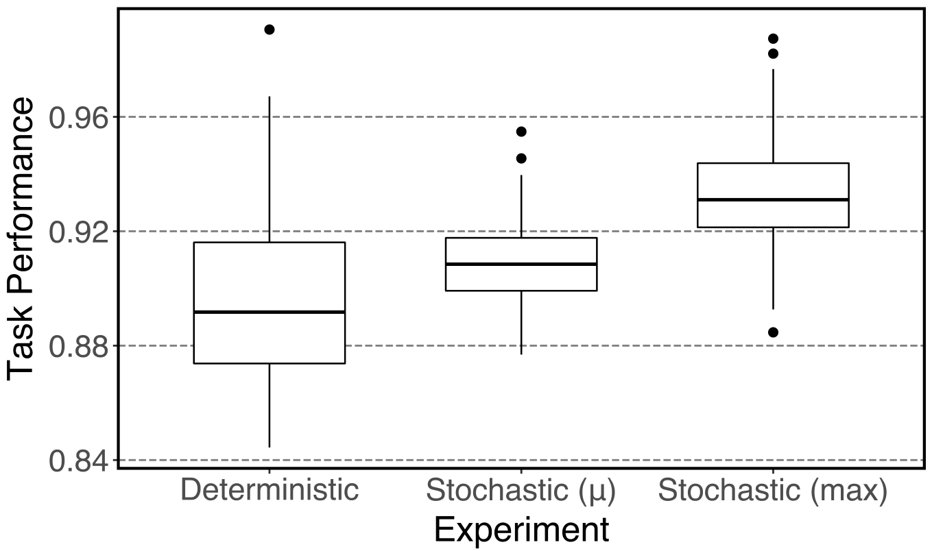
Table 2 presents four RC metrics of the fittest reservoirs. As expected, the control group’s metrics are worse¹ than those of the task-grown reservoirs. The 100-node experiment shows considerably higher Generalisation Rank (GR) and Linear Memory Capacity (LMC). Stochastic reservoirs show the highest Kernel Rank (KR) and a very low GR relative to their

Figure 9: Samples of recurring structures. tanh neurons are shown in black and linear neurons in gray. Negative $(-1)$negative one weights are shown in red. Reservoirs grown for the NARMA task exhibit “life-like” structural motifs, reminiscent of biological networks (Milo et al., 2002)as described by Milo and colleagues in 2002. The diversity of these structures suggests that the DGCA model is capable of generating specialised networks with functional properties characteristic of natural systems.

performance. Despite the high SR spread, both the deterministic 100-node and stochastic 200-node reservoirs show a median SR of $0$zero. This might suggest a prevalence of acyclic structures, as these topologies have all Eigenvalues equal to $0$zero.

4.1.1 Structures

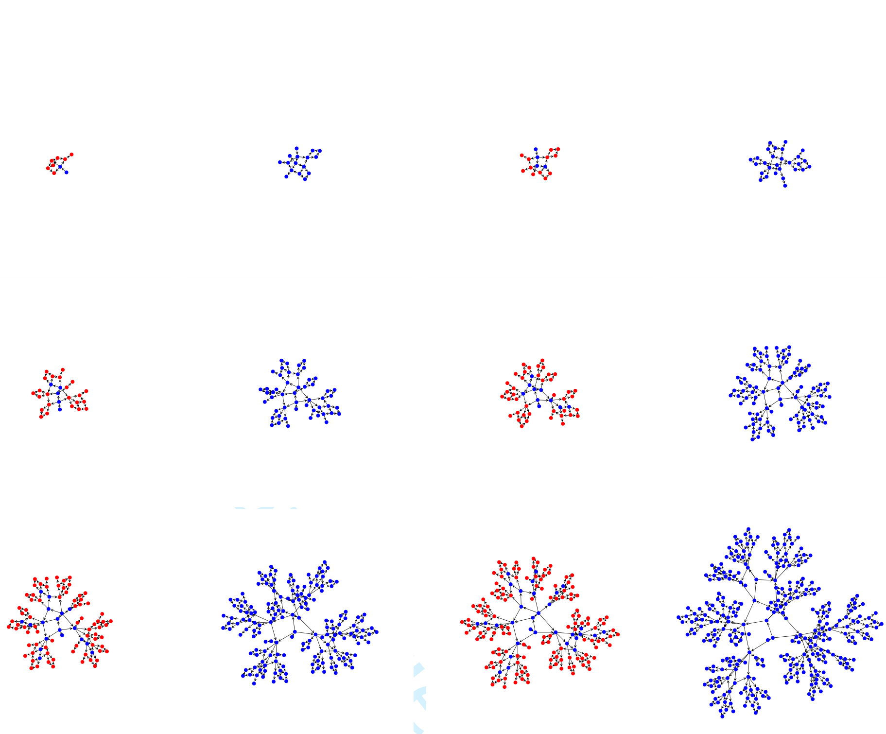
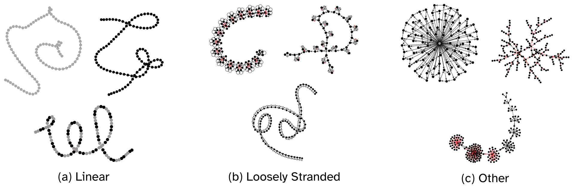
We observed that grown reservoirs tend to converge on a set of distinct topological patterns. To investigate whether there is a relationship between structure and performance, we classify the grown reservoirs into three categories. Many of the observed structures contained linear strands or strand-like characteristics. Figure 9 shows some sample reservoirs grown during the study, while illustrating the three categories into which the reservoirs were classified for subsequent analysis. Graphs are visualised using the graph-tool² library.

• Linear includes all graphs that form unbranched strands of nodes. Graphs with isolated chains (e.g. two disconnected strands) also fall under this category.
• The Loosely Stranded category includes all graphs that follow a strand-like structure but with additional complexity. These typically include double strands with con

nections between nodes of opposite strands, and strands with self-loops or cyclic subgraphs.

• Other includes all remaining structures. These can be described as tree-like, clustered, hubs, among others. Unlike the previous two, no single dominant pattern emerged.

To systematically classify the graphs, we use three graph metrics: betweenness centrality, closeness centrality, and diameter (Hagberg et al., 2007)as described by Hagberg and colleagues (see Equations 3, 4, 5 respectively). For a graph $G=(V,E)$G equals V, E with $n=|V|$n equals the number of vertices in V, the betweenness centrality of a node $v\in V$v in V is defined as

where ${\sigma }_{st}$ is the number of shortest paths between nodes $s$ and $t$, and ${\sigma }_{st}(v)$ is the number of those paths that pass through $v$. When normalised (as in this study), this quantity is divided by $(n-1)(n-2)/2$. The closeness centrality of a node $v$ is defined as

where $d(v,u)$ is the shortest-path distance between $v$ and $u$. The diameter of a network is

that is, the maximum shortest-path distance between any pair of nodes.

We first treat each graph as undirected and decompose it into its connected components. For each component, we compute these three metrics. We use the 90th percentile of node betweenness centrality within a component to capture nodes that may serve as structural bridges, the median closeness centrality to summarise the overall efficiency of information

Figure 10: Pairwise relationships between graph metrics used for clustering: 90th percentile betweenness centrality, median closeness centrality, and normalised diameter. Each point represents a reservoir. colours indicate the $k=3$k equals three clusters identified by K-means.

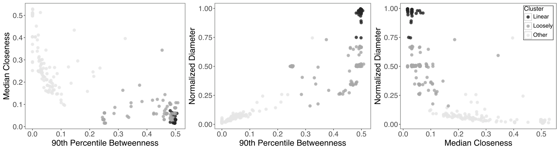
reach, and the diameter normalised by component size to characterise how extended the component is. We then compute a size-weighted average of these quantities across all components of a graph, assigning greater influence to larger components. This procedure yields three aggregate values per graph, one for each metric. We then applied K-means clustering to partition the graphs into $k=3$k equals three clusters (see Figure 10).

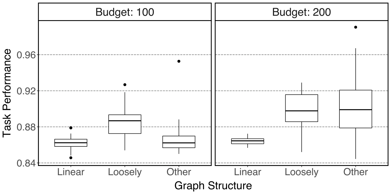
Figure 11 presents the distribution of task performance split by structure. In the 100-node experiment, Loosely Stranded graphs perform significantly better than the other two categories. In the 200-node experiments, Loosely Stranded and Other structures achieve the highest performance, while Linear graphs consistently rank the lowest. These results suggest that under tighter resource constraints (i.e. reduced node budgets), Loosely Stranded graphs provide an advantage.

Under constrained budgets, Linear reservoirs are the most prevalent structure $\approx 47\%$approximately 47 percent, as expected from the median Spectral Radius (SR) of $0$zero (see Table 2). For larger budgets, Other becomes the most prevalent category $\approx 59\%$approximately 59 percent. This suggests that a larger budget enables more structural diversity, while a smaller one favours simpler, reliable solutions.

To better understand the role of individual nodes within each structure, we performed node ablation experiments. For each reservoir, we prune nodes individually one at a time and

Figure 11: Structural distribution of task performance across node budgets. Pairwise comparisons used independent two-sample U-tests with Bonferroni correction $\alpha =0.05$alpha equals zero point zero five, corrected threshold $p<0.0167$p less than zero point zero one six seven. Significant differences, 100-node: Loosely Stranded vs Linear ($p=3.012e-13$p equals three point zero one two times ten to the minus thirteen), Loosely Stranded vs Other ($p=1.319e-7$p equals one point three one nine times ten to the minus seven). Significant differences, 200-node: Linear vs Other ($p=1.169e-7$p equals one point one six nine times ten to the minus seven), Linear vs Loosely Stranded ($p=5.993e-8$p equals five point nine nine three times ten to the minus eight).

312 record the change in task performance relative to the baseline. We then restore the node 313 before the next ablation. Figure 12 shows representative node ablation patterns for the 314 three emerging structures. The Linear reservoir’s ablation confirms that NARMA is pre-315 dominantly a memory task, evidenced by the blue-red-blue pattern. Pruning nodes near 316 the middle of the strand causes the greatest drop in performance, as it truncates the ef-317 fective memory span of the reservoir. The Loosely Stranded “double helix” shows no clear 318 pattern of node importance. This makes the topology more robust than the linear one, 319 since the redundant and parallel pathways mean that no single node is solely responsible 320 for transmitting information. Lastly, the Other example reveals the fragility of hub struc-321 tures. The central hub node mediates the flow of information between a large portion of 322 the network, making it a critical bottleneck whose removal greatly disrupts reservoir per-323 formance.

324 While Stochastic reservoirs have a median SR of $0$zero (see Table 2), none grew into linear 325 structures. In fact, all reservoirs produced in the stochastic experiment belong to the Other 326 structural category. Approximately 70% have underlying Directed Acyclic Graphs (DAGs), 327 which explains the low median SR. As shown in Figure 13, the DAGs exhibit different levels

Figure 12: Representative examples of node ablation patterns across reservoir structures. For each reservoir, nodes are individually pruned one at a time, the change in task performance relative to the baseline is recorded, and the node is then restored before the next ablation. Node colour encodes the resulting performance difference ($\Delta$delta), with red indicating greater performance degradation and blue indicating minimal impact.

Figure 13: Samples of stochastic directed acyclic reservoirs with increasing connectivity. Mean degree (edges per node): 2.8 (low), 4.8 (medium), and 7.3 (high).

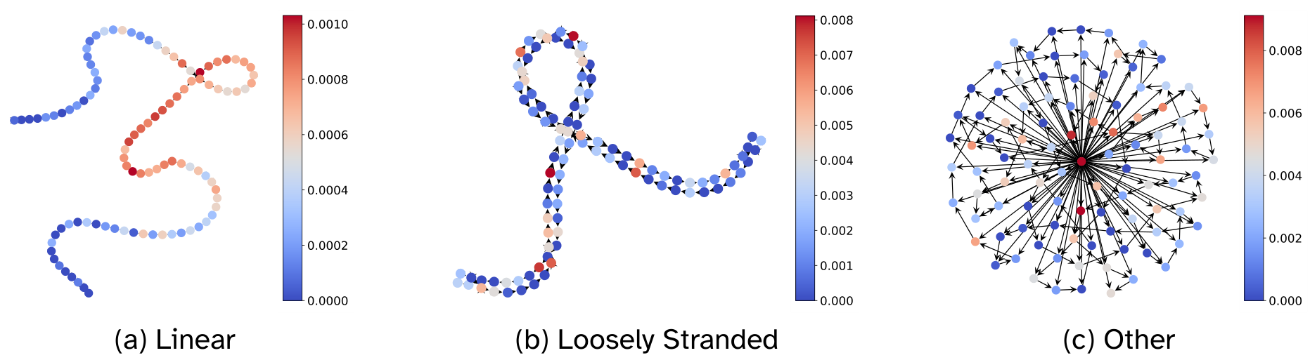
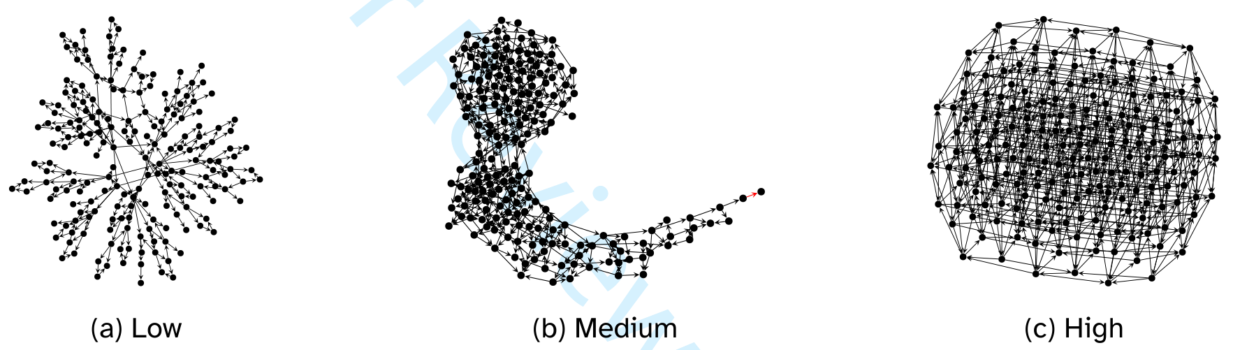
of connectivity, but almost all reservoirs (cyclic and acyclic) are fairly similar to one of the three showcased topologies.

To better understand the Stochastic structures, we looked into the graph metrics used previously for classification, as well as three additional ones: mean node degree, average path length, and degree assortativity (Hagberg et al., 2007)Hagberg and colleagues, 2007. Mean node degree measures the average number of edges connected to each node in the graph. Average path length measures the mean number of steps along the shortest paths between all pairs of nodes. Degree assortativity measures the tendency of nodes to connect with other nodes that have similar degrees. Table 3 shows that the range and types of Stochastic structures are fundamentally different from their Deterministic counterparts. Stochastic reservoirs have

Table 3: Graph metrics of deterministic and stochastic reservoirs. Degree, betweenness, and closeness are averaged over nodes within each reservoir. Assortativity is measured with respect to node degree. Values are reported as median (interquartile range).

338 approximately twice the connectivity (5.97 vs 3.08)5.97 versus 3.08. More edges mean each node 339 integrates more signals per timestep. The median and interquartile range (IQR) difference in 340 average path length indicates that Stochastic structures are consistently more compact. 341 The high IQR for Deterministic average path length (1.05 vs 29.54)1.05 versus 29.54 reflects that these 342 experiments explore a structurally diverse set of solutions, while Stochastic experiments 343 tend to converge to one regime. Similarly, the high IQR for Deterministic diameter (89.25) 344 means some reservoirs are extremely elongated (strands), while others are more compact. 345 The difference in median closeness centrality (0.24 vs 0.15)0.24 versus 0.15 also indicates that, in Stochastic 346 reservoirs, nodes are much closer to all other nodes on average. Stochastic reservoirs 347 are also more assortative, where highly connected nodes cluster together and peripheral 348 nodes connect to the core. Deterministic assortativity is closer to 0, meaning connectivity 349 is more evenly distributed (with a few exceptions, IQR = 0.41I Q R equals 0.41). Finally, the wider spread of 350 betweenness centrality (0.006 vs 0.013)0.006 versus 0.013 confirms that some Deterministic reservoirs have 351 extreme bottleneck nodes (hubs), a non-existent phenomenon in Stochastic reservoirs.

4.2 Task-Driven Growth: NARMA-N

353 To evaluate the adaptability of DGCA under increasing task difficulty, we grew an additional 354 300 reservoirs with higher NARMA orders. We tested for $N=20$N equals 20 and $N=30$N equals 30 tasks 355 with a fixed budget of 200 nodes and deterministic sensing. As expected, increasing task 356 difficulty leads to a decrease in performance. Figure 14 shows performance distributions 357 across NARMA orders and reservoir structures. The procedure described in Section 4.1.1 358 was also used to classify the reservoirs of the new experiments. For NARMA-20, Loosely

Figure 14: Structural distribution of task performance across NARMA orders. NARMA-10 results are reproduced from Figure 11 for reference. DGCAs are given a budget of 200 nodes. Pairwise comparisons used independent two-sample U-tests with Bonferroni correction ($\alpha =0.05$alpha equals zero point zero five, corrected threshold $p<0.0167$p less than zero point zero one six seven). Significant differences, NARMA-20: Linear vs Loosely Stranded ($p=1.691e-8$p equals one point six nine one times ten to the minus eight), Loosely Stranded vs Other ($p=2.482e-3$p equals two point four eight two times ten to the minus three). Significant differences, NARMA-30: Linear vs Loosely Stranded ($p=3.724e-9$p equals three point seven two four times ten to the minus nine), Linear vs Other ($p=2.430e-3$p equals two point four three zero times ten to the minus three).

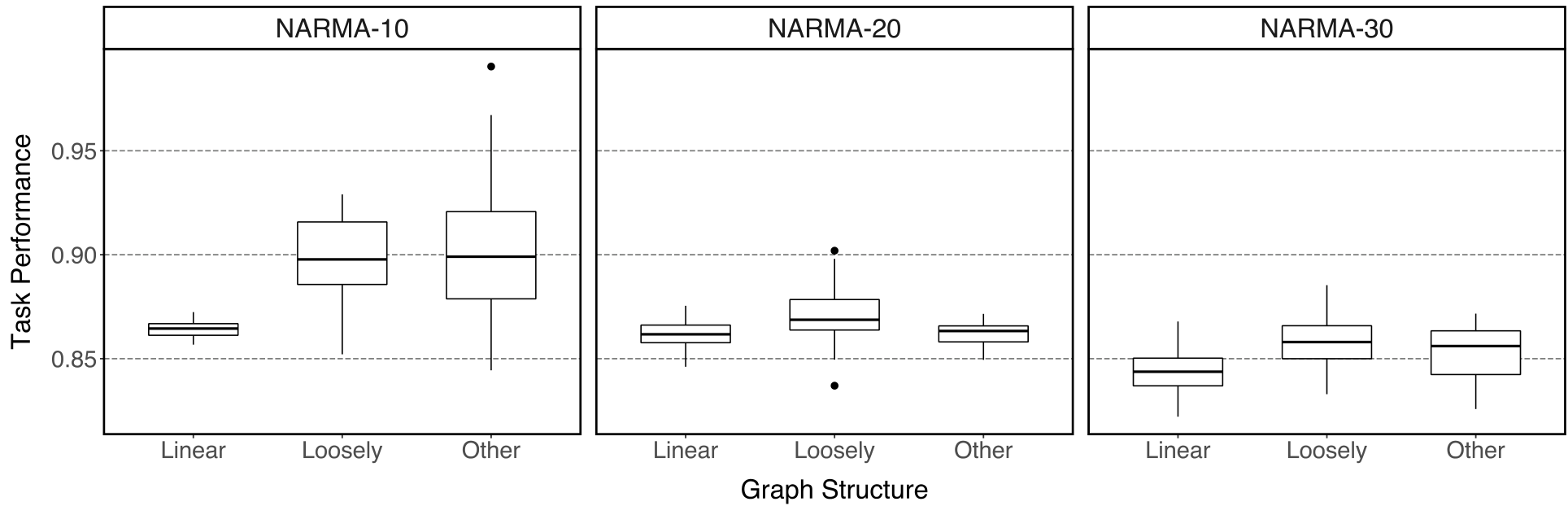
Stranded reservoirs outperform the other two categories, with no significant difference between Linear and Other. For NARMA-30, Linear performs the worst, and Loosely Stranded reservoirs exhibit the highest median performance (not significant).

Table 4 shows the RC metrics of the fittest reservoirs across NARMA orders. A median SR of 1 across all experiments indicates that Linear structures are uncommon among successful solutions. GR and LMC show substantial improvement when moving from NARMA-10 to the more difficult NARMA-20 and NARMA-30 tasks. This suggests that these two metrics may play a critical role in supporting reservoir performance under increasing NARMA complexity. Despite not explicitly optimising for GR or LMC, the DGCA is able to specialise in ways that prioritise these metrics as task difficulty increases.

4.3 Task-Independent Growth

While we have shown that a reservoir can be grown to solve specific tasks by training directly on them, we now ask whether optimising for task-independent properties (KR, GR,

Table 4: Task-independent properties of NARMA-$N$N grown reservoirs. Values are reported as median (interquartile range). Each row represents a different NARMA-$N$N experiment, while each column corresponds to a metric computed from the fittest reservoirs. Kernel Rank (KR), Generalisation Rank (GR) and Linear Memory Capacity (LMC) are normalised by the number of nodes.

etc.) can yield reservoirs that generalise to unseen tasks. We set the DGCA’s fitness function to each metric individually, as well as to an additive combination of all four. All experiments were conducted with a 200-node budget.

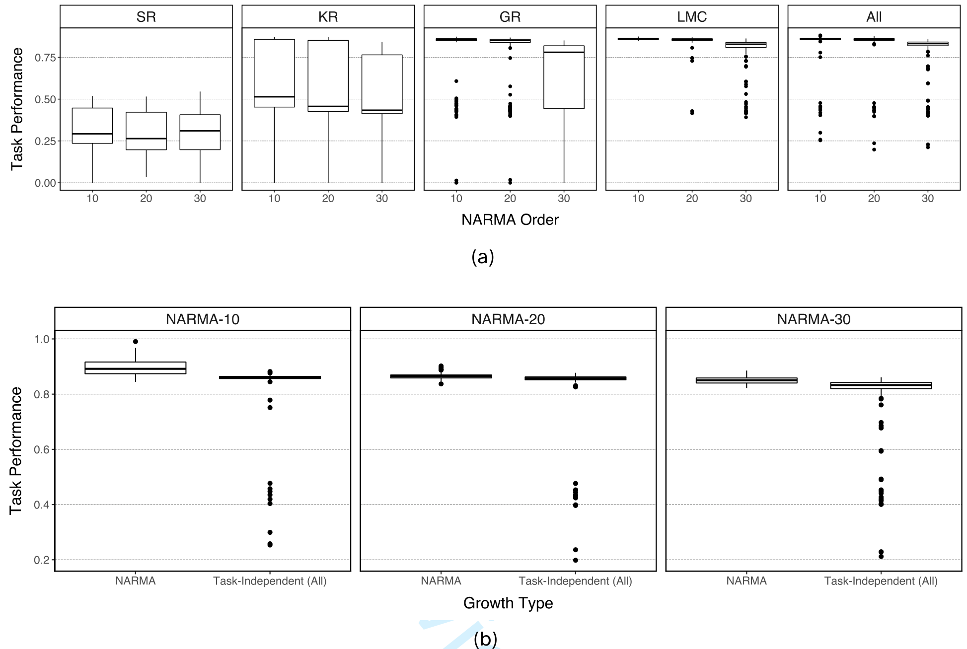
Figure 15a shows task performance across different target metrics and NARMA orders. GR and LMC are the most effective approximators of task performance (after All). SR is the worst-performing target metric across all NARMA orders, followed by KR. The spread in task performance for KR-grown reservoirs is relatively high, suggesting that this metric is less robust than GR or LMC and may lead to unpredictable behaviour in NARMA tasks.

Figure 15b compares task performance distributions of task-grown (NARMA) and metric-grown (All) reservoirs. Note that the same task-independent reservoirs are used across all NARMA orders, whereas task-grown ones are tailored to each. Perhaps unsurprisingly, task-specific growth yields a significant performance improvement over the more general, metric-based approach. Notably, however, reservoirs grown using these metrics alone still perform well, despite the fact that such metrics are only indirect proxies of reservoir dynamics.

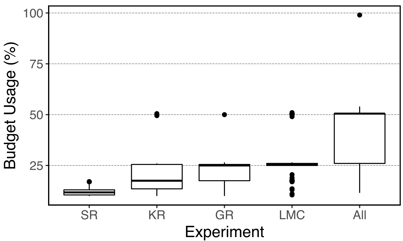
Figure 16 shows budget usage (%) across the different metric-based experiments. In contrast to task-grown reservoirs, metric-grown reservoirs tend to use fewer neurons. The All experiment uses the most ($\approx$50%approximately 50 percent), while LMC uses only around 25%.

Table 5 shows the RC metrics of the fittest metric-grown reservoirs. GR and LMC experi-

Figure 15: Task performance distribution across growth type, NARMA orders and metrics. The chosen metrics are: Spectral Radius (SR), Kernel Rank (KR), Generalisation Rank (GR), and Linear Memory Capacity (LMC). DGCAs are given a budget of 200 nodes. (a) Task performance comparison across metric and NARMA order. (b) Task performance comparison across growth types. Pairwise comparisons used independent two-sample U-tests with Bonferroni correction ($\alpha =0.05$alpha equals zero point zero five, corrected threshold $p<0.0167$p less than zero point zero one six seven). Significant differences: NARMA-10 ($p=9.613e-36$p equals nine point six one three times ten to the minus thirty six), NARMA-20 ($p=1.994e-13$p equals one point nine nine four times ten to the minus thirteen), NARMA-30 ($p=3.378e-23$p equals three point three seven eight times ten to the minus twenty three).

ments produce reservoirs ‘competitive’ with task-grown ones. SR is $0$zero for both, suggesting that this metric is less relevant in the context of NARMA tasks. These scores, however, do not suggest that LMC or GR alone are exclusive predictors of NARMA performance, as earlier experiments showed that reservoirs with significantly lower memory capacity ($\approx 30\%$approximately thirty percent of LMC) or generalisation potential ($\approx 40\%$approximately forty percent of GR) were consistently able to outperform those with higher scores (see Table 4).

Figure 16: Distribution of budget usage (%) across task-independent properties.

Table 5: Task-independent properties of metric-grown reservoirs. Values are reported as median (interquartile range). Each row represents a different task-independent experiment, while each column corresponds to a metric computed from the fittest reservoirs. Kernel Rank (KR), Generalisation Rank (GR) and Linear Memory Capacity (LMC) are normalised by the number of nodes.

5 Discussion

In this paper, we have demonstrated that DGCAs can be used to grow reservoirs. We have used an adaptation of the Microbial Genetic Algorithm (MGA) to find the neural network weights of DGCAs based on fitness functions centred around task performance and RC metrics. The grown reservoirs were then benchmarked against imitation tasks of increasing difficulty.

The structural diversity of the produced reservoirs indicates that distinct graph configurations can emerge as viable solutions to the same problem. Among these, some low-density,

linear strand topologies emerged as the best performing. This finding suggests that even resource limited, sparse networks can function as effective reservoirs. Moreover, recurring “life-like” structures proved to be consistently better performing than others across experiments. These are, for all practical purposes, unachievable by the search of randomly-generated networks, as these often result in small-world reservoirs.

Griffin et al. (2026)Griffin and colleagues show that Echo State Networks (ESNs) using tanh neurons can be approximated by simple time-lagged systems, suggesting that linear regression on the output does most of the heavy lifting. The development of linear strand reservoirs with only linear neurons (see Figure 9a) supports this idea, as they perform comparably to tanh strand reservoirs. We propose two explanations for the emergence of these linear systems. First, linear neurons may simply be sufficient for the task, and the evolutionary algorithm converged on them as an effective solution. Second, it is not unheard of for evolutionary algorithms to creatively subvert intentions by exploiting unrecognised bugs in code or producing unexpected adaptations (Lehman et al., 2020)as noted by Lehman and colleagues. A decision made during implementation was to clamp all arithmetic overflow reservoir states. Unsurprisingly, chains of linear activations can produce these overflows, and the clamping may introduce an artificial source of non-linearity. After further investigation, we observed one case of clamping, where the effect was minimal (1.3% of activations clamped), meaning we can confidently say this has not impacted the results presented.

Adding stochasticity to the DGCA growth process aided in finding genotypes capable of producing better performing reservoirs. We believe the randomness introduced in the cells’ sensing phase acts as a form of canalisation (Waddington, 1942)as described by Waddington, preventing genotypes from exploiting precise (and brittle; see Figure 12) configurations. Since cells acted on inaccurate environmental information, only genotypes that reliably produced well performing structures across several stochastic growth instances could survive selection. This might have smoothed the fitness landscape, with a bias toward a consistently compact

structural regime rather than the diverse topological solutions found under deterministic growth. Interestingly, the majority of stochastically grown reservoirs were acyclic, with a spectral radius of $0$zero. This warrants further investigation, as it challenges the conventional assumption that a spectral radius close to $1$one is a prerequisite for effective reservoir dynamics.

Growing reservoirs based on RC metrics alone demonstrates that some of these can serve as reasonable approximators of task performance. However, task-grown reservoirs also occasionally exhibit relatively high task performance despite having modest scores across all four inspected metrics. These counterexamples suggest that standard RC metrics may not fully capture or predict task performance, pointing to the need for a broader theoretical framework to understand what makes a reservoir effective.

This work lays the foundation for the development of a DGCA capable of producing plastic reservoirs—structures that can grow and repair themselves—bringing us a step closer to modeling a robust computational system akin to biological life. Such reservoirs are particularly valuable in remote-location applications or embedded systems, where structural damage or changes in task demands may occur. In such scenarios, traditional fixed-structure reservoirs lack a recovery mechanism, requiring total replacement instead of self-repair or adaptation. Future work could explore artificial perturbations or task redefinitions to evaluate the system’s potential for continual learning.

Given that DGCAs were designed as a model for directed graph growth, the integration of a RC context also opens new avenues for research along these lines. We are looking towards integrating Liquid State Machines (spiking neural network versions of reservoir computers) and a broader task domain.

Simulating physical reservoirs is common practice in theoretical research, particularly in the early stages of developing ideas. At the experimental level, however, challenges remain in mapping RC simulated models to physical systems. First, it may be unrealistic to perturb

the entire system (i.e. input weights connected to all nodes). Second, it is often infeasible to observe the full state of the substrate. Inspired by physical reservoir computing, we have begun developing an input-output scheme that defines a fixed set of input and output nodes. In this setup, the reservoir grows around the fixed input and output neurons, similar to the use of probes in physical substrates (Cai et al., 2023)as shown by Cai and colleagues in 2023.

Future work could also investigate the relationship between reservoir topology and reservoir dynamics using network reconstruction techniques (Peixoto, 2025)by Peixoto or sub-graph extraction techniques (Welke et al., 2018)by Welke and colleagues. By inferring structures from the reservoir’s internal state, it may be possible to identify functional motifs, explain performance differences between structures, and even develop more informative task-independent measures of computational capacity.

One of the disadvantages of using DGCAs to produce reservoirs is the slow training or optimisation of neural network weights. Due to the lack of a differentiable update function, adjusting weights must rely on search-based methods rather than the more efficient gradient-based optimisation. We are actively designing a differentiable version of the model using Graph Neural Networks. We are also looking at the role of different activation functions (Griffin et al., 2026)as discussed by Griffin and colleagues, and how these might influence the behaviour of the grown reservoirs.

To conclude, we have demonstrated the ability of DGCAs to grow reservoirs. Our results, evaluated using task- and metric-based fitness functions, highlight the model’s potential in reservoir computing. This work contributes to the advancement of DGCAs as a viable framework for reservoir computing and opens new directions for modelling morphogenesis inspired by nature’s purposeful growth.

6 Acknowledgements

We would like to thank Riversdale Waldegrave, author of the original DGCA model, for helpful discussions during the early stages of this work.

Code available at: GitHub.

References

Aven, T., Jensen, J. H., & Tufte, G. (2024). Lattice reservoirs: Symmetry breaking and information flow in physical reservoir computing. Artificial Life Conference Proceedings 36, 2024(1), 49.

Bengio, Y., Simard, P., & Frasconi, P. (1994). Learning long-term dependencies with gradient descent is difficult. IEEE transactions on neural networks, 5(2), 157–166.

Cai, H., Ao, Z., Tian, C., Wu, Z., Liu, H., Tchieu, J., Gu, M., Mackie, K., & Guo, F. (2023). Brain organoid reservoir computing for artificial intelligence. Nature Electronics, 6(12), 1032–1039.

Dale, M., Miller, J. F., Stepney, S., & Trefzer, M. A. (2019). A substrate-independent framework to characterize reservoir computers. Proceedings of the Royal Society A: Mathematical, Physical and Engineering Sciences, 475(2226), 20180723. https://doi.org/10.1098/rspa.2018.0723

Galbraith, M., Bocci, F., & Onuchic, J. N. (2022). Stochastic fluctuations promote ordered pattern formation of cells in the notch-delta signaling pathway. PLOS Computational Biology, 18(7), e1010306.

Grattarola, D., Livi, L., & Alippi, C. (2021). Learning graph cellular automata. Advances in Neural Information Processing Systems, 34, 20983–20994.

Griffin, D., Stovold, J., O’Keefe, S., & Stepney, S. (2026). Evaluating ESNs Against Lagged Input Regression Computation. In E. Formenti & L. Manzoni (Eds.), Unconventional