Pretraining Recurrent Networks without Recurrence
Akarsh Kumar
Phillip Isola
MIT
Abstract
Training recurrent neural networks (RNNs) requires assigning credit across long sequences of computations. Standard backpropagation through time (BPTT) addresses this problem poorly: it is sequential in time, limiting parallelism, and suffers from vanishing or exploding gradients, making long-range associations difficult to learn. We propose Supervised Memory Training (SMT), a method for training nonlinear RNNs that sidesteps recurrent credit propagation entirely by reducing RNN training to supervised learning on one-step memory transition labels
GRAY
Project Page: akarshkumar.com/smt
Source Code: github.com/akarshkumar0101/smt
1 Introduction
Recurrent neural networks (RNNs) store information about the past that will only become useful in the future. The core training challenge is that the utility of a memory may be delayed: many intermediate computations intervene between writing information and eventually using it. These intervening steps confound learning the correct associations, a problem known as credit assignment
The standard approach, backpropagation through time (BPTT), assigns credit across a sequence by unrolling the RNN in time and propagating gradients backward through the resulting computation graph
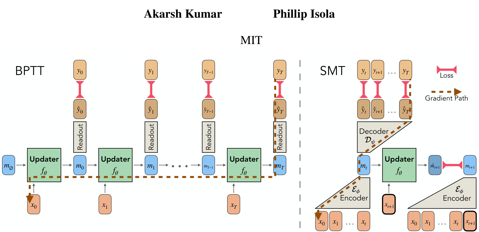
In this paper, we propose Supervised Memory Training (SMT), a method to train nonlinear RNNs that sidesteps recurrent credit propagation by reducing the problem to supervised learning. Suppose we had access to the optimal memory state at each timestep,
The challenge, of course, is how to actually obtain such memory labels. In this paper, we assert that an effective memory is a sufficient statistic of the past for predicting the future, i.e., a predictive state
In practice, we train a Transformer encoder model to embed the past context into a memory that a separate decoder can use to predict the future. This objective operationalizes the notion of a predictive state: a representation of the past that retains only the information needed to predict the future and nothing more. Once this teacher encoder has learned to construct such memory representations, the RNN can then focus on learning the now much simpler task of updating that memory over time.
In essence, SMT decouples learning what to remember (memory representation), which is a non-sequential problem, from learning how to update memory (memory dynamics), which is a sequential process but can be supervised one-step at a time. This decoupling enables time-parallel training of nonlinear RNNs without unrolling, and creates a stable
Indeed, Transformers solved time-parallelism and credit assignment in the same way
Linear attention RNN models also exhibit time-parallel training and relatively stable credit assignment, while maintaining a fixed memory size
SMT aims to combine the best of all worlds: time-parallel training, stable
2 Methods
2.1 Background
Causal Conditional Sequence Modeling Let
Recurrent Neural Networks (RNNs) An RNN models this problem using a fixed-size latent state,
where
Backpropagation Through Time (BPTT) Traditionally, RNNs are trained with BPTT
Gradients are then computed end-to-end on this unrolled computation graph, propagating from the output prediction losses backward through the trajectory of the nonlinear dynamical system. Thus, this gradient credit assignment signal may have to travel for a path length of up to
BPTT has two well-known limitations:
- Equation 1 is usually implemented with a recurrent for-loop, preventing parallelization
[97] . - BPTT often produces unstable high variance gradients
[11] . When gradients vanish, the RNN experiences a recency bias, hindering the learning of long-range associations[101] . When gradients explode, the induced dynamical system is chaotic, causing training instability[98] .
2.2 Supervised Memory Training (SMT)
We propose Supervised Memory Training (SMT) for pretraining nonlinear RNNs without BPTT. The core idea is to decouple the learning of memory representation from memory dynamics.
Motivation Consider a hypothetical oracle memory-encoding model
In practice, SMT approximates
Formulation Formally, we have the RNN
The encoder maps each context to a memory state with
The future decoding loss for timestep
We have the RNN predict the next memory given the current memory and the next input with
This dynamics loss has two distinct purposes: 1) to train the RNN and 2) to explicitly shape the encoder memory representations to be Markovian (i.e.
We add a uniformity loss
The full objective is a weighted sum of all three losses:
where the
Practice Theoretically, it should be enough to train
For experiments, we truncate
Properties of SMT In SMT, the encoder model constructs appropriate memory representations of the past, while the RNN is responsible for learning the now much simpler task of updating that memory in one-step, thereby decoupling memory representation from memory dynamics. In contrast, under BPTT training, the RNN must learn both tasks simultaneously. Since the memory labels are acquired with a “teacher” encoder-decoder pair, SMT inherits all of its properties, such as time-parallelism,
2.3 DAgger Memory Training (DMT)
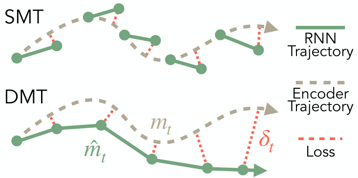
After SMT, the RNN achieves low one-step error in predicting
We introduce DAgger Memory Training (DMT), a finetuning phase that corrects this drift via on-policy imitation learning
Concretely, given
During DMT, we freeze the encoder and decoder and only train the RNN with a small learning rate.
Note that DMT unrolls the RNN memories, but still uses teacher forced
unrolls the RNN and gradients may optionally propagate through time, its objective is fundamentally
different than standard BPTT, since long-range credit is already assigned in the encoder memory
labels,
fine-tuning phase following SMT. Table 1 shows the resource requirements for the different methods.
| Training (-Length Sequence) | Inference (One-Step) | Complexity Class | |||||
|---|---|---|---|---|---|---|---|
| Method | Memory | Compute | Sequential Operations | Credit Path Length | Memory | Compute | |
| Transformer | |||||||
| LA (parallel) | |||||||
| LA (recurrent) | |||||||
| BPTT (RNN) | L/P | ||||||
| SMT (RNN) | L/P | ||||||
| DMT (RNN) | L/P |
3 Experiments
We study the properties of SMT and compare against BPTT, the standard RNN training algorithm.
We restrict our analysis to nonlinear RNNs, the primarily setting BPTT is applied. Transformers and
linear RNNs are excluded as they are qualitatively distinct model classes
“BPTT RNN” denotes the BPTT baseline. “SMT Encoder*” generates memories
baseline with the same memory bottleneck as our RNNs. Since it serves as the teacher during SMT
and DMT, it provides a reference upper bound on RNN performance. “SMT DMT RNN” denotes
the RNN pretrained with SMT and finetuned with DMT, which constitutes our full method.
Architectures We use RNN architectures based on a Transformer, MLP, and GRU
Datasets We consider character-level language modeling on TinyStories
task requiring long-range memory
raster-scan order pixel sequence modeling of sparse images from MNIST
This is a hard problem for RNNs
pixel, row by row. When you see a new white pixel, in order to recognize the shape and slope of the
stroke it belongs to, you must remember the white pixels you saw in the previous rows, which may be
hundreds of timesteps ago, buried among black pixels. RNNs must achieve this with finite memory,
meaning no direct attention to earlier pixels, and thus forcing long-range memory to emerge. We
term this “Attneave’s task”, based on classic work from perceptual psychology
More details on architectures, datasets, and experiments are in Appendix B.
3.1 Synthetic Task Experiments
We first evaluate BPTT and SMT on synthetic tasks designed to isolate and probe specific properties
of the training algorithm. The RNN architecture with the Transformer backbone is used for these
experiments. For these synthetic experiments, we set
expected value. Our tasks include the following (details of tasks are in Appendix B.2.1):
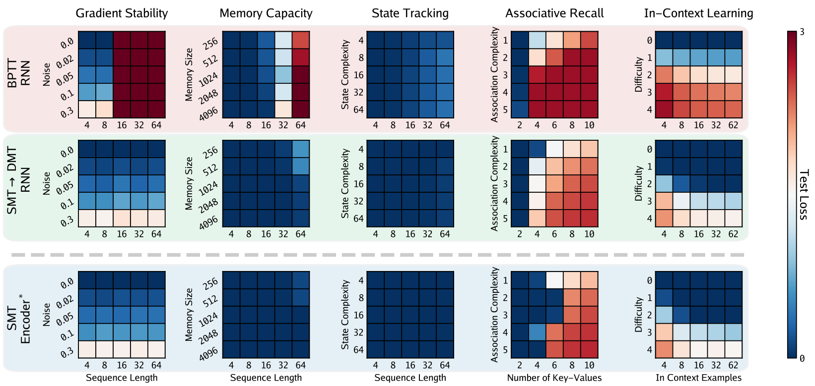
- Retrieval to test Gradient Stability (sweep sequence length and noise level).
- String Copy to test Memory Capacity (sweep sequence length and memory state size).
- Stack Operations to test State Tracking (sweep sequence length and state complexity).
- Keys-Values to test Associative Recall (sweep number of and complexity of associations).
- Modular Arithmetic to test In-Context Learning (sweep difficulty and number of examples).
Figure 3 shows that SMT DMT outperforms BPTT in all settings of all tasks. BPTT struggles to
learn as sequences get longer, even when the task is simple, e.g. retrieval. It also struggles to utilize
memory capacity fully, do associative recall, and perform in-context learning, all of which require
solving long-range credit assignment. In contrast, SMT seems agnostic to the sequence length, and
is able to solve all of the harder credit assignment problems except associative recall. We attribute
these differences to BPTT’s
Section 3.7 confirms the difference in gradient stability in both methods.
3.2 Attneave’s Pixel Sequence Modeling
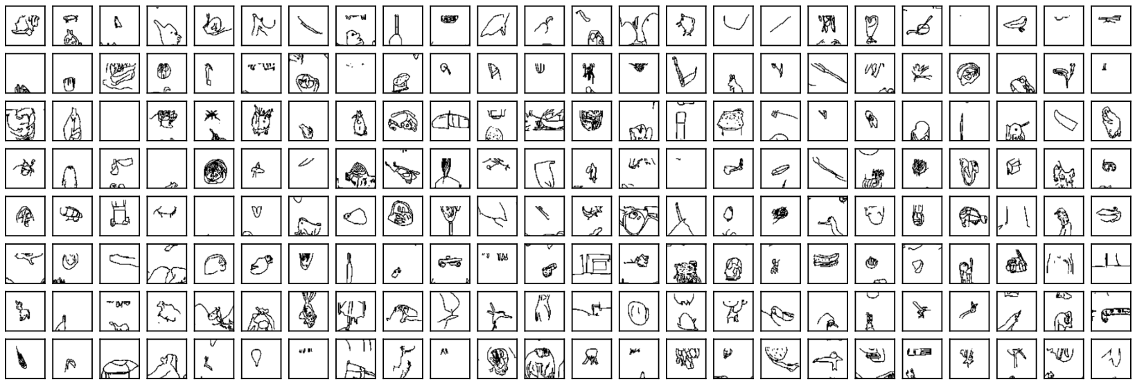
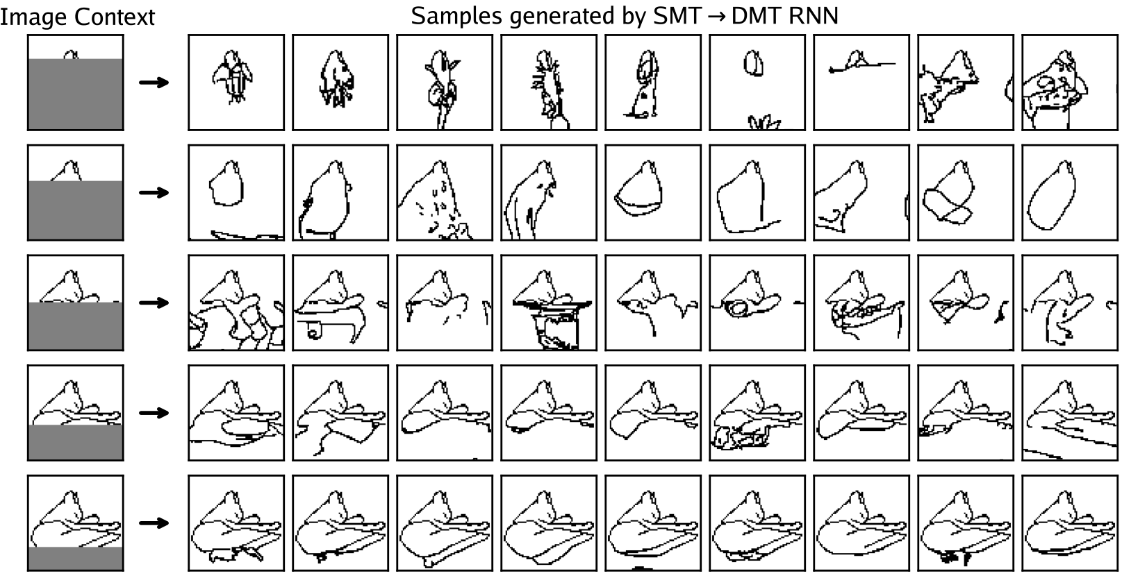
We now evaluate on Attneave’s tasks. Figure 4 shows the stark difference between MNIST samples generated by RNNs trained with BPTT and SMTDMT. Figure 5 shows images generated by an SMTDMT RNN trained on Sketchy.
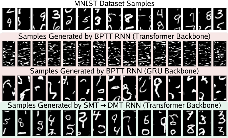
Along with the synthetic experiments, these results confirm that SMT doesn’t suffer from a recency bias like BPTT, allowing it to properly attribute credit across long sequences.
3.3 Sequential Compute and Data
We now evaluate BPTT and SMT across real domains and various RNN architectures. Each method is allowed
Figure 6 shows the results. In sequential compute, SMT Encoder and SMTDMT RNN are significantly more efficient than BPTT with the Transformer and MLP backbones. In data, SMT Encoder and SMTDMT RNN has approximately
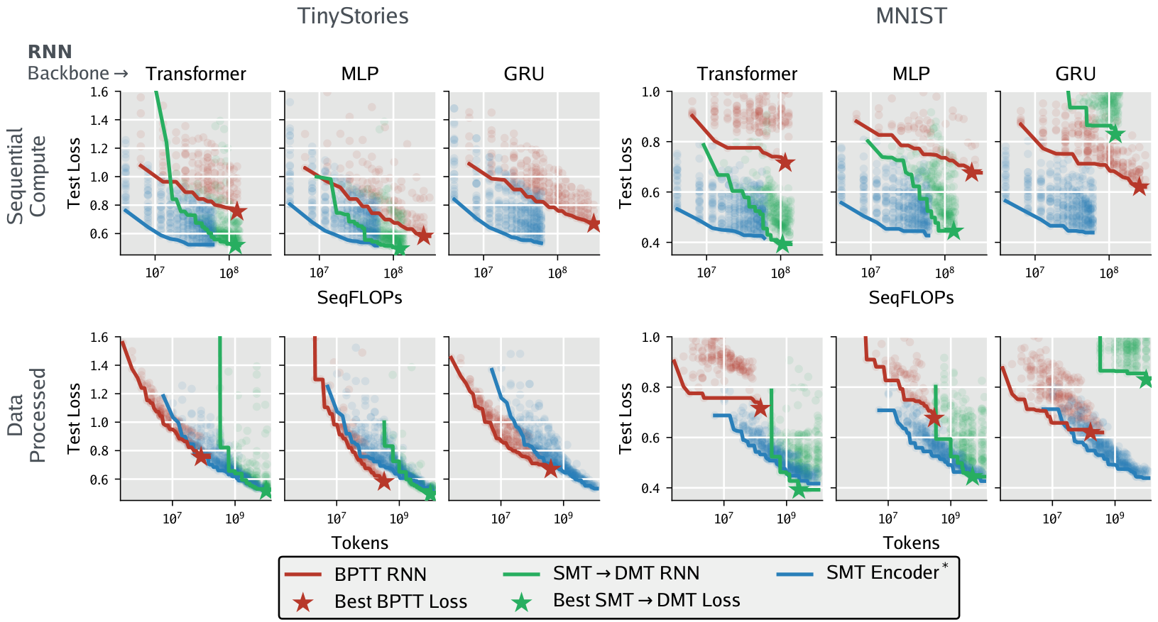
the same data efficiency as BPTT with the Transformer and MLP backbones on TinyStories. However on MNIST, SMT Encoder and SMTDMT RNN shows significantly better data efficiency. This result is explained by the short vs long range memory information requirements of natural language
3.4 Scaling Laws
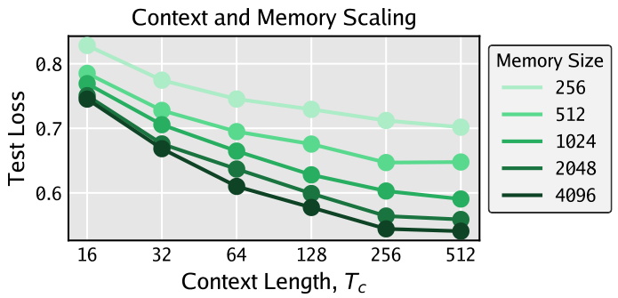
We evaluate the scaling behavior of SMTDMT along three axes: context length, memory state size, and model parameter count. For the first two, we logarithmically sweep
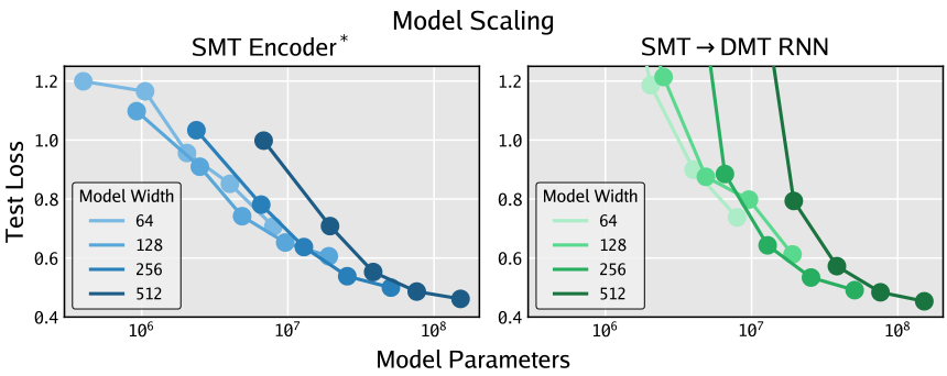
Figure 7 shows that SMTDMT exhibits smooth, predictable performance improvements with larger context length and bigger memory state size. Together with the previous experiments, these results reaffirm that SMT effectively leverages long contexts and large memory states. Figure 8 presents the parameter scaling results. The SMT encoder follows a standard power-law-like scaling trend. The SMTDMT RNN also improves smoothly with scale, albeit with a differently shaped scaling curve. Interestingly, the RNN appears to more closely match the encoder’s performance at larger scales.
3.5 Compression as a Scaling Axis
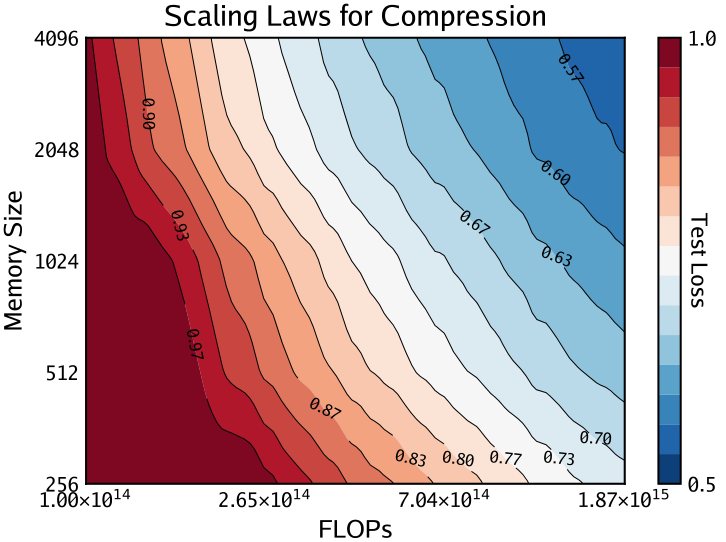
Neural scaling laws predict the relationship between a resource
Figure 9 shows the scaling curve, confirming that SMT can achieve more compression when allocated more compute. Since compression is often speculated as being a core property of intelligent systems
3.6 Ablations
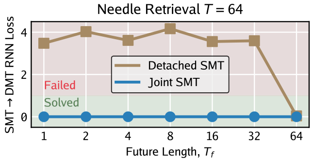
Predictive State and Detached RNN The impact of the predictive state objective (Equation 2) is evaluated by sweeping the future length
Figure 10 shows the results on the needle retrieval task. To solve the task, and thus have proper credit assignment, SMT requires either large enough
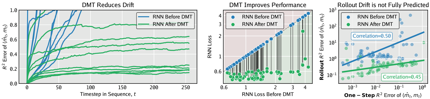
Drift and DMT As described in Section 2.3, RNN suffers from drift post-SMT. Figure 12 shows an analysis of drift and DMT’s mitigation of it. From a dynamical systems perspective, DMT seems to discover RNNs which have an initially higher drift, but which plateau at a much lower equilibrium drift. Interestingly, this equilibrium drift value is not fully predicted by the one-step drift, inviting future investigations into predicting and mitigating rollout drift in one-step during SMT.
3.7 Analysis
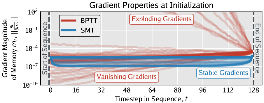
Gradient Properties of BPTT and SMT The fundamental difference between BPTT and SMT in long-range credit assignment is dictated by their gradients. Figure 11 shows the gradient magnitude of ,
Benefit of RNNs over Transformers SMT trains an RNN to mimic a Transformer encoder model, raising the question of why an RNN is needed at all, given the Transformer. RNNs are qualitatively more efficient than Transformers at inference, requiring
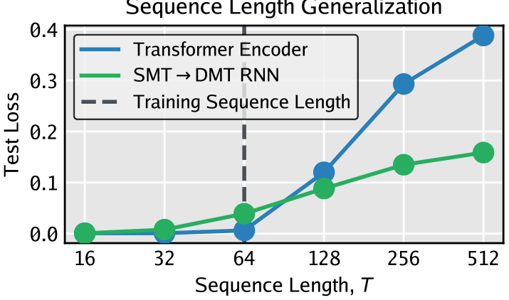
Here, we compare an SMTDMT RNN against a Transformer on the synthetic stack state tracking task. For a fair comparison, we use the SMT encoder as the Transformer baseline, since it imposes the same memory-information bottleneck as the RNN.
Figure 13 shows the Transformer outperforms the RNN on training sequence lengths, but significantly underperforms the RNN on sequence lengths longer than training. Prior work on length generalization reports similar findings
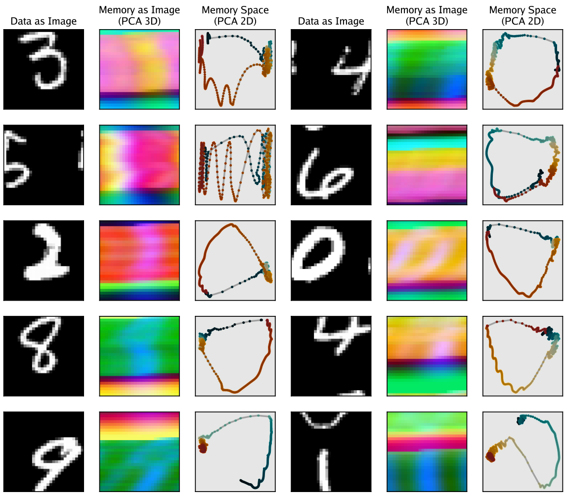
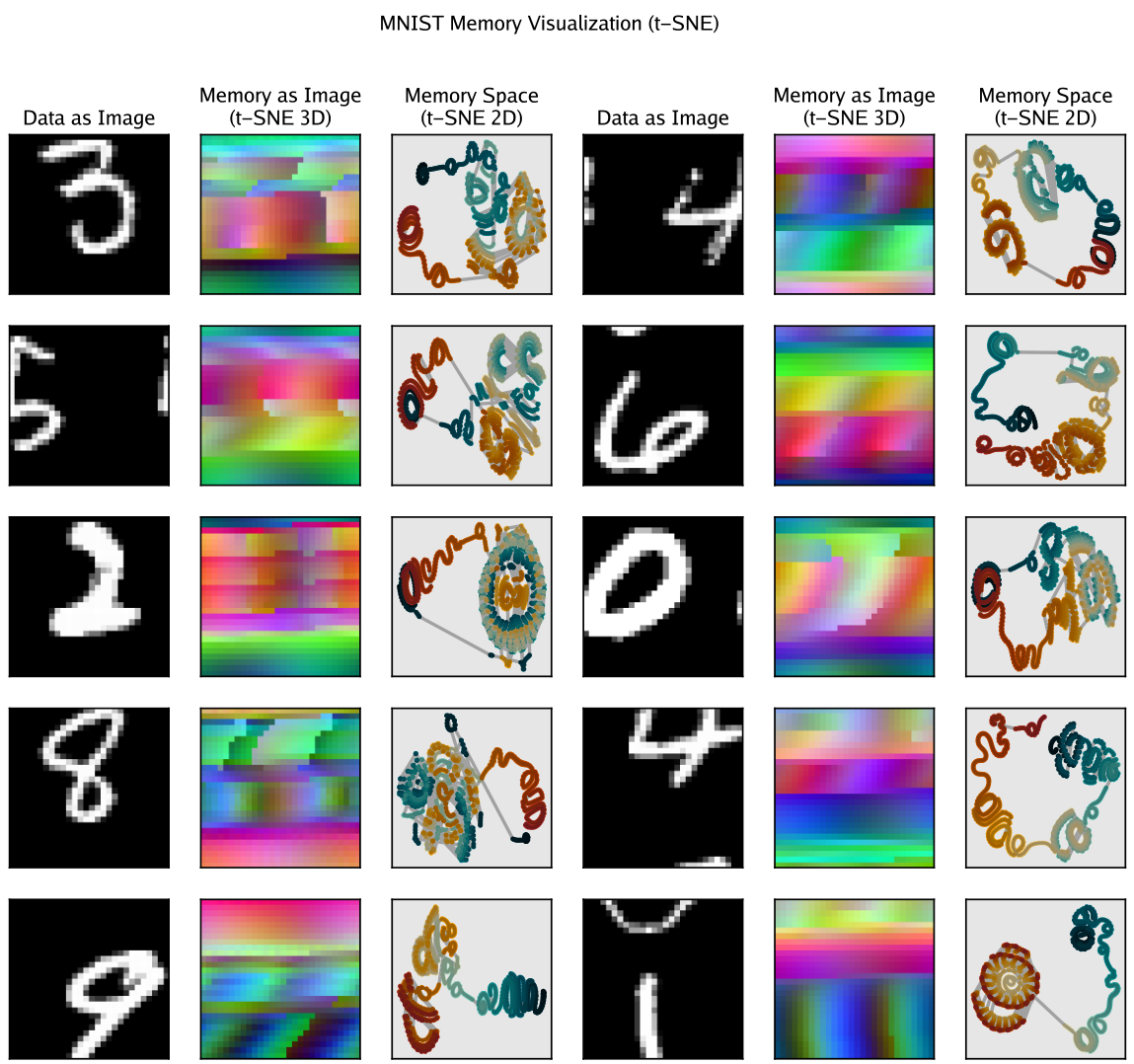
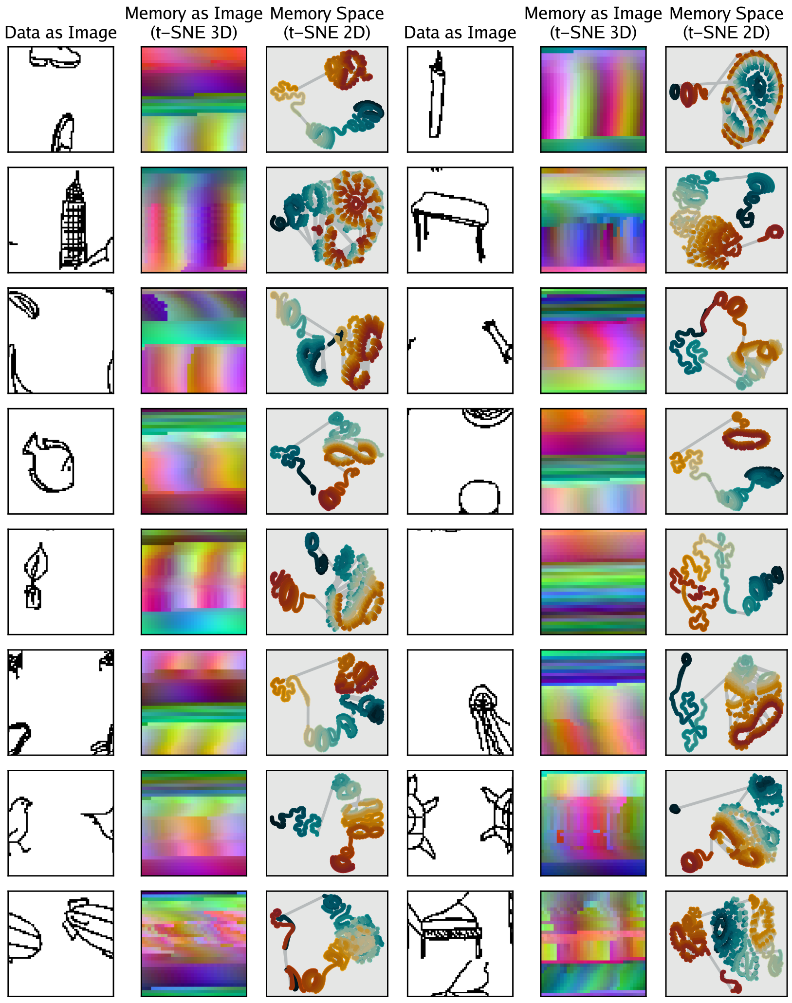
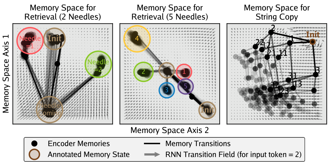
Memory Space To better understand what SMT is learning, we train smaller SMT models that have a 2D memory state and directly visualize their memory space across three synthetic tasks in Figure 14. In the retrieval tasks, SMT learns to collapse many sequence states into only a few effective memory states: an initial state, a state indicating the next token is the needle, and states corresponding to the needle value. Then, the RNN learns finite-state machine behavior to transition between these states. In contrast, string copying requires lossless sequence compression and thus SMT cannot alias distinct memory states together. It learns to create a tree-like memory geometry to store all possible sequences, matching the tree structure of all possible strings. Figure 21 and Figure 22 show memory visualizations for models trained on MNIST. These results indicate SMT memories form effective temporal abstractions of the past depending on what the future requires.
4 Related Works
Relation with NextLat Highly related and concurrent to our work,
Recurrent Neural Networks (RNNs) RNNs were studied extensively early in AI because their recurrence mechanism resembles biological brains
However, it has repeatedly been shown that BPTT produces unstable gradients that vanish, explode, or exhibit high variance
Recently, there has been renewed interest in RNNs in the form of linear state space models
Time-Parallel Training Transformers revolutionized sequence modeling
A recent line of work attempts to parallelize nonlinear RNNs as well
Computation Complexity Class of Models A model’s architecture determines the problems it can theoretically solve
and linear RNNs, are provably limited to tasks with equivalently low circuit depth
In SMT, we train a nonlinear RNN (which is fully expressive), using a time-parallel teacher Transformer (which has limits). We note this limitation but argue that SMT is a pretraining algorithm, which should be used with a lightweight post-training algorithm to solve downstream tasks
Predictive State Representations (PSRs) A PSR is a way of modeling a partially observed dynamical system by representing its state only in terms of predictions about future observations
PSRs have been previously incorporated into RNNs
Other Related Work Our work is related to the literature on cross-architecture teacher-student distillation
5 Discussion
In SMT, the teacher model is time-parallel, and is thus constrained in expressivity
The current SMT variant computes and trains only a single
RNNs have the promise of solving problems that extend over unbounded horizons, such as the entire lifetime of an agent. However, training methods for RNN have been hindered by the inability of BPTT to assign credit effectively over such a long horizon. Our method circumvents the credit assignment issue with an
Acknowledgments and Disclosure of Funding
References
[2] Gene M Amdahl. Validity of the single processor approach to achieving large scale computing capabilities. In Proceedings of the April 18-20, 1967, spring joint computer conference, pages 483–485, 1967.
[3] Peter J Angeline, Gregory M Saunders, and Jordan B Pollack. An evolutionary algorithm that constructs recurrent neural networks. IEEE transactions on Neural Networks, 5(1):54–65, 1994.
[4] Martin Arjovsky, Amar Shah, and Yoshua Bengio. Unitary evolution recurrent neural networks. In International conference on machine learning, pages 1120–1128. PMLR, 2016.
[5] Fred Attneave. Some informational aspects of visual perception. Psychological review, 61(3): 183, 1954.
[6] Dzmitry Bahdanau, Kyunghyun Cho, and Yoshua Bengio. Neural machine translation by jointly learning to align and translate, 2016. URL arXiv.
[7] Shaojie Bai, J Zico Kolter, and Vladlen Koltun. An empirical evaluation of generic convolutional and recurrent networks for sequence modeling. arXiv, 2018.
[8] Shaojie Bai, J Zico Kolter, and Vladlen Koltun. Deep equilibrium models. Advances in neural information processing systems, 32, 2019.
[9] Maximilian Beck, Korbinian Pöppel, Markus Spanring, Andreas Auer, Oleksandra Prudnikova, Michael Kopp, Günter Klambauer, Johannes Brandstetter, and Sepp Hochreiter. xlstm: Extended long short-term memory. Advances in Neural Information Processing Systems, 37: 107547–107603, 2024.
[10] Samy Bengio, Oriol Vinyals, Navdeep Jaitly, and Noam Shazeer. Scheduled sampling for sequence prediction with recurrent neural networks, 2015. URL arXiv.
[11] Yoshua Bengio, Patrice Simard, and Paolo Frasconi. Learning long-term dependencies with gradient descent is difficult. IEEE transactions on neural networks, 5(2):157–166, 1994.
[12] Max S Bennett. A brief history of intelligence: evolution, AI, and the five breakthroughs that made our brains. HarperCollins, 2023.
[13] Guy E Blelloch. Prefix sums and their applications. 1990.
[14] Tom Brown, Benjamin Mann, Nick Ryder, Melanie Subbiah, Jared D Kaplan, Prafulla Dhariwal, Arvind Neelakantan, Pranav Shyam, Girish Sastry, Amanda Askell, et al. Language models are few-shot learners. Advances in neural information processing systems, 33:1877–1901, 2020.
[16] Yingfa Chen, Zhen Leng Thai, Zihan Zhou, Zhu Zhang, Xingyu Shen, Shuo Wang, Chaojun Xiao, Xu Han, and Zhiyuan Liu. Hybrid linear attention done right: Efficient distillation and effective architectures for extremely long contexts, 2026. URL arXiv.
[17] Kyunghyun Cho, Bart Van Merriënboer, Dzmitry Bahdanau, and Yoshua Bengio. On the properties of neural machine translation: Encoder–decoder approaches. In Proceedings of SSST-8, eighth workshop on syntax, semantics and structure in statistical translation, pages 103–111, 2014.
[18] Junyoung Chung, Caglar Gulcehre, KyungHyun Cho, and Yoshua Bengio. Empirical evaluation of gated recurrent neural networks on sequence modeling. arXiv preprint arXiv:1412.3555, 2014.
[19] Junyoung Chung, Sungjin Ahn, and Yoshua Bengio. Hierarchical multiscale recurrent neural networks. arXiv preprint arXiv:1609.01704, 2016.
[20] Stephen A Cook. A taxonomy of problems with fast parallel algorithms. Information and control, 64(1-3):2–22, 1985.
[21] Zihang Dai, Zhilin Yang, Yiming Yang, Jaime G Carbonell, Quoc Le, and Ruslan Salakhutdinov. Transformer-xl: Attentive language models beyond a fixed-length context. In Proceedings of the 57th annual meeting of the association for computational linguistics, pages 2978–2988, 2019.
[22] Federico Danieli, Miguel Sarabia, Xavier Suau Cuadros, Pau Rodriguez, and Luca Zappella. Deeppcr: Parallelizing sequential operations in neural networks. Advances in Neural Information Processing Systems, 36:47598–47625, 2023.
[23] Federico Danieli, Pau Rodriguez, Miguel Sarabia, Xavier Suau, and Luca Zappella. Pararnn: Unlocking parallel training of nonlinear rnns for large language models, 2025. URL arXiv.
[24] Tri Dao and Albert Gu. Transformers are ssms: Generalized models and efficient algorithms through structured state space duality. arXiv preprint arXiv:2405.21060, 2024.
[25] Carlton Downey, Ahmed Hefny, and Geoffrey Gordon. Practical learning of predictive state representations. arXiv preprint arXiv:1702.04121, 2017.
[26] Carlton Downey, Ahmed Hefny, Boyue Li, Byron Boots, and Geoffrey Gordon. Predictive state recurrent neural networks, 2017. URL arXiv.
[27] Ronen Eldan and Yuanzhi Li. Tinystories: How small can language models be and still speak coherent english? arXiv preprint arXiv:2305.07759, 2023.
[28] Jeffrey L Elman. Finding structure in time. Cognitive science, 14(2):179–211, 1990.
[29] Angela Fan, Thibaut Lavril, Edouard Grave, Armand Joulin, and Sainbayar Sukhbaatar. Addressing some limitations of transformers with feedback memory. arXiv preprint arXiv:2002.09402, 2020.
[30] Lizhe Fang, Yifei Wang, Zhaoyang Liu, Chenheng Zhang, Stefanie Jegelka, Jinyang Gao, Bolin Ding, and Yisen Wang. What is wrong with perplexity for long-context language modeling?, 2025. URL arXiv.
[31] Leo Feng, Frederick Tung, Mohamed Osama Ahmed, Yoshua Bengio, and Hossein Hajimirsadeghi. Were rnns all we needed? arXiv preprint arXiv:2410.01201, 2024.
[32] Yulu Gan and Phillip Isola. Neural thickets: Diverse task experts are dense around pretrained weights. arXiv preprint arXiv:2603.12228, 2026.
[34] Angeliki Giannou, Shashank Rajput, Jy-yong Sohn, Kangwook Lee, Jason D Lee, and Dimitris Papailiopoulos. Looped transformers as programmable computers. In International Conference on Machine Learning, pages 11398–11442. PMLR, 2023.
[35] Xavier Gonzalez, Andrew Warrington, Jimmy T Smith, and Scott W Linderman. Towards scalable and stable parallelization of nonlinear rnns. Advances in Neural Information Processing Systems, 37:5817–5849, 2024.
[36] Xavier Gonzalez, Leo Kozachkov, David M Zoltowski, Kenneth L Clarkson, and Scott W Linderman. Predictability enables parallelization of nonlinear state space models. arXiv, 2025.
[37] Alex Graves, Greg Wayne, and Ivo Danihelka. Neural turing machines. arXiv, 2014.
[38] Albert Gu. On the tradeoffs of state space models and transformers, 2025. URL goombalab.github.io.
[39] Albert Gu and Tri Dao. Mamba: Linear-time sequence modeling with selective state spaces. arXiv, 2023.
[40] Albert Gu, Karan Goel, and Christopher Ré. Efficiently modeling long sequences with structured state spaces. arXiv, 2021.
[41] Steven Stenberg Hansen. Long timescale credit assignment in neuralnetworks with external memory, 2017. URL arXiv.
[42] Shibo Hao, Sainbayar Sukhbaatar, DiJia Su, Xian Li, Zhiting Hu, Jason Weston, and Yuandong Tian. Training large language models to reason in a continuous latent space, 2025. URL arXiv.
[43] Lukas Hauzenberger, Niklas Schmidinger, Thomas Schmied, Anamaria-Roberta Hartl, David Stap, Pieter-Jan Hoedt, Maximilian Beck, Sebastian Böck, Günter Klambauer, and Sepp Hochreiter. Effective distillation to hybrid xlstm architectures, 2026. URL arXiv.
[44] Kaiming He, Xiangyu Zhang, Shaoqing Ren, and Jian Sun. Deep residual learning for image recognition. In Proceedings of the IEEE conference on computer vision and pattern recognition, pages 770–778, 2016.
[45] Donald Olding Hebb. The organization of behavior: A neuropsychological theory. Psychology press, 1949.
[46] Ahmed Hefny, Zita Marinho, Wen Sun, Siddhartha Srinivasa, and Geoffrey Gordon. Recurrent predictive state policy networks, 2018. URL arXiv.
[47] Kyle Helfrich, Devin Willmott, and Qiang Ye. Orthogonal recurrent neural networks with scaled cayley transform. In International Conference on Machine Learning, pages 1969–1978. PMLR, 2018.
[48] Salah Hihi and Yoshua Bengio. Hierarchical recurrent neural networks for long-term dependencies. Advances in neural information processing systems, 8, 1995.
[49] W Daniel Hillis and Guy L Steele Jr. Data parallel algorithms. Communications of the ACM, 29(12):1170–1183, 1986.
[50] Geoffrey E Hinton and James A Anderson. Parallel models of associative memory: updated edition. Psychology press, 2014.
[52] Sepp Hochreiter and Jürgen Schmidhuber. Long short-term memory. Neural computation, 9 (8):1735–1780, 1997.
[53] Sepp Hochreiter, Yoshua Bengio, Paolo Frasconi, Jürgen Schmidhuber, et al. Gradient flow in recurrent nets: the difficulty of learning long-term dependencies, 2001.
[54] Jordan Hoffmann, Sebastian Borgeaud, Arthur Mensch, Elena Buchatskaya, Trevor Cai, Eliza Rutherford, DDL Casas, Lisa Anne Hendricks, Johannes Welbl, Aidan Clark, et al. Training compute-optimal large language models. arXiv, 10, 2022.
[55] Sara Hooker. The hardware lottery. Communications of the ACM, 64(12):58–65, 2021.
[56] John J Hopfield. Neural networks and physical systems with emergent collective computational abilities. Proceedings of the national academy of sciences, 79(8):2554–2558, 1982.
[57] Kurt Hornik, Maxwell Stinchcombe, and Halbert White. Multilayer feedforward networks are universal approximators. Neural networks, 2(5):359–366, 1989.
[58] Edward S Hu, Kwangjun Ahn, Qinghua Liu, Haoran Xu, Manan Tomar, Ada Langford, Dinesh Jayaraman, Alex Lamb, and John Langford. Learning to achieve goals with belief state transformers. arXiv, 2024.
[59] Marcus Hutter. Universal artificial intelligence: Sequential decisions based on algorithmic probability, volume 300. Springer, 2005.
[60] Mozes Jacobs, Thomas Fel, Richard Hakim, Alessandra Brondetta, Demba Ba, and T Andy Keller. Block-recurrent dynamics in vision transformers. arXiv, 2025.
[61] Herbert Jaeger. The “echo state” approach to analysing and training recurrent neural networks-with an erratum note. Bonn, Germany: German national research center for information technology gmd technical report, 148(34):13, 2001.
[62] Alexia Jolicoeur-Martineau. Less is more: Recursive reasoning with tiny networks, 2025. URL arXiv.
[63] Leslie Pack Kaelbling, Michael L Littman, and Anthony R Cassandra. Planning and acting in partially observable stochastic domains. Artificial intelligence, 101(1-2):99–134, 1998.
[64] Anil Kag and Venkatesh Saligrama. Training recurrent neural networks via forward propagation through time. In International Conference on Machine Learning, pages 5189–5200. PMLR, 2021.
[65] Eric R Kandel. Principles of neural science, 2000.
[66] Jared Kaplan, Sam McCandlish, Tom Henighan, Tom B Brown, Benjamin Chess, Rewon Child, Scott Gray, Alec Radford, Jeffrey Wu, and Dario Amodei. Scaling laws for neural language models. arXiv, 2020.
[67] Jungo Kasai, Hao Peng, Yizhe Zhang, Dani Yogatama, Gabriel Ilharco, Nikolaos Pappas, Yi Mao, Weizhu Chen, and Noah A. Smith. Finetuning pretrained transformers into rnns, 2021. URL arXiv.
[68] Angelos Katharopoulos, Apoorv Vyas, Nikolaos Pappas, and François Fleuret. Transformers are rnns: Fast autoregressive transformers with linear attention. In International conference on machine learning, pages 5156–5165. PMLR, 2020.
[69] Louis Kirsch, James Harrison, Jascha Sohl-Dickstein, and Luke Metz. General-purpose in-context learning by meta-learning transformers. arXiv, 2022.
[70] Andrei Nikolaevic Kolmogorov. Three approaches to the quantitative definition of information. International journal of computer mathematics, 2(1-4):157–168, 1968.
[72] Yann LeCun and Corinna Cortes. The MNIST database of handwritten digits, 1998. URL http://yann.lecun.com/exdb/mnist/.
[73] Belinda Z. Li, Zifan Carl Guo, and Jacob Andreas. (how) do language models track state?, 2025. URL arXiv.
[74] Qinyu Li, Yee Whye Teh, and Razvan Pascanu. Noprop: Training neural networks without full back-propagation or full forward-propagation. arXiv, 2025.
[75] Yi Heng Lim, Qi Zhu, Joshua Selfridge, and Muhammad Firmansyah Kasim. Parallelizing non-linear sequential models over the sequence length, 2024. URL arXiv.
[76] Michael Littman and Richard S Sutton. Predictive representations of state. Advances in neural information processing systems, 14, 2001.
[77] Bingbin Liu, Jordan T Ash, Surbhi Goel, Akshay Krishnamurthy, and Cyril Zhang. Transformers learn shortcuts to automata. arXiv, 2022.
[78] Yuxi Liu, Konpat Preechakul, Kananart Kuwaranancharoen, and Yutong Bai. The serial scaling hypothesis. arXiv, 2025.
[79] Mantas Lukoševičius and Herbert Jaeger. Reservoir computing approaches to recurrent neural network training. Computer science review, 3(3):127–149, 2009.
[80] Eric Martin and Chris Cundy. Parallelizing linear recurrent neural nets over sequence length, 2018. URL arXiv.
[81] Warren S McCulloch and Walter Pitts. A logical calculus of the ideas immanent in nervous activity. The bulletin of mathematical biophysics, 5(4):115–133, 1943.
[82] William Merrill and Ashish Sabharwal. The parallelism tradeoff: Limitations of log-precision transformers. Transactions of the Association for Computational Linguistics, 11:531–545, 2023.
[83] William Merrill and Ashish Sabharwal. The expressive power of transformers with chain of thought, 2024. URL arXiv.
[84] William Merrill, Jackson Petty, and Ashish Sabharwal. The illusion of state in state-space models. arXiv, 2024.
[85] William Merrill, Hongjian Jiang, Yanhong Li, and Ashish Sabharwal. Why are linear rnns more parallelizable? arXiv, 2026.
[86] Zakaria Mhammedi, Andrew Hellicar, Ashfaqur Rahman, and James Bailey. Efficient orthogonal parametrisation of recurrent neural networks using householder reflections. In International Conference on Machine Learning, pages 2401–2409. PMLR, 2017.
[87] Thomas Miconi, Jeff Clune, and Kenneth O. Stanley. Differentiable plasticity: training plastic neural networks with backpropagation, 2018. URL arXiv.
[88] Geoffrey F Miller, Peter M Todd, and Shailesh U Hegde. Designing neural networks using genetic algorithms. In ICGA, volume 89, pages 379–384, 1989.
[89] John Miller and Moritz Hardt. Stable recurrent models. arXiv, 2018.
[90] Marvin Minsky. Steps toward artificial intelligence. Proceedings of the IRE, 49(1):8–30, 1961.
[91] Mayank Mishra, Shawn Tan, Ion Stoica, Joseph Gonzalez, and Tri Dao. M2 rnn: Nonlinear rnns with matrix-valued states for scalable language modeling. arXiv, 2026.
[93] Elias Najarro and Sebastian Risi. Meta-learning through hebbian plasticity in random networks, 2022. arXiv.
[94] Yann Ollivier, Corentin Tallec, and Guillaume Charpiat. Training recurrent networks online without backtracking. arXiv, 2015.
[95] Costin-Andrei Oncescu, Depen Morwani, Samy Jelassi, Alexandru Meterez, Mujin Kwun, and Sham Kakade. The recurrent transformer: Greater effective depth and efficient decoding. arXiv, 2026.
[96] James M Ortega and Werner C Rheinboldt. Iterative solution of nonlinear equations in several variables. SIAM, 2000.
[97] Razvan Pascanu, Caglar Gulcehre, Kyunghyun Cho, and Yoshua Bengio. How to construct deep recurrent neural networks. arXiv, 2013.
[98] Razvan Pascanu, Tomas Mikolov, and Yoshua Bengio. On the difficulty of training recurrent neural networks. In International conference on machine learning, pages 1310–1318. Pmlr, 2013.
[99] Leonid Peshkin, Nicolas Meuleau, and Leslie Kaelbling. Learning policies with external memory. arXiv, 2001.
[100] Ofir Press, Noah A Smith, and Mike Lewis. Train short, test long: Attention with linear biases enables input length extrapolation. arXiv, 2021.
[101] Shauli Ravfogel, Yoav Goldberg, and Tal Linzen. Studying the inductive biases of rnns with synthetic variations of natural languages. In Proceedings of the 2019 Conference of the North American Chapter of the Association for Computational Linguistics: Human Language Technologies, Volume 1 (Long and Short Papers), pages 3532–3542, 2019.
[102] Stephane Ross, Geoffrey J. Gordon, and J. Andrew Bagnell. A reduction of imitation learning and structured prediction to no-regret online learning, 2011. arXiv.
[103] David E Rumelhart, Geoffrey E Hinton, and Ronald J Williams. Learning representations by back-propagating errors. nature, 323(6088):533–536, 1986.
[104] Walter L Ruzzo. On uniform circuit complexity. Journal of Computer and System Sciences, 22(3):365–383, 1981.
[105] Tim Salimans, Jonathan Ho, Xi Chen, Szymon Sidor, and Ilya Sutskever. Evolution strategies as a scalable alternative to reinforcement learning. arXiv, 2017.
[106] Patsorn Sangkloy, Nathan Burnell, Cusuh Ham, and James Hays. The sketchy database: learning to retrieve badly drawn bunnies. Acm Transactions on Graphics (TOG), 35(4):1–12, 2016.
[107] Bidipta Sarkar, Mattie Fellows, Juan Agustin Duque, Alistair Letcher, Antonio León Villares, Anya Sims, Clarisse Wibault, Dmitry Samsonov, Dylan Cope, Jarek Liesen, et al. Evolution strategies at the hyperscale. arXiv, 2025.
[108] Andrew M Saxe, James L McClelland, and Surya Ganguli. Exact solutions to the nonlinear dynamics of learning in deep linear neural networks. arXiv, 2013.
[109] Jürgen Schmidhuber, Sepp Hochreiter, and Yoshua Bengio. Evaluating benchmark problems by random guessing. A Field Guide to Dynamical Recurrent Networks, pages 231–235, 2001.
[110] Makoto Shing, Masanori Koyama, and Takuya Akiba. Diffusionblocks: Block-wise neural network training via diffusion interpretation. arXiv, 2025.
[112] Satinder P Singh, Michael L Littman, Nicholas K Jong, David Pardoe, and Peter Stone. Learning predictive state representations. In Proceedings of the 20th International Conference on Machine Learning (ICML-03), pages 712–719, 2003.
[113] Jimmy TH Smith, Andrew Warrington, and Scott W Linderman. Simplified state space layers for sequence modeling. arXiv, 2022.
[114] Ray J Solomonoff. A formal theory of inductive inference. part i. Information and control, 7 (1):1–22, 1964.
[115] Rupesh Kumar Srivastava, Klaus Greff, and Jürgen Schmidhuber. Highway networks. arXiv, 2015.
[116] Kenneth O Stanley and Risto Miikkulainen. Evolving neural networks through augmenting topologies. Evolutionary computation, 10(2):99–127, 2002.
[117] Jianlin Su, Murtadha Ahmed, Yu Lu, Shengfeng Pan, Wen Bo, and Yunfeng Liu. Roformer: Enhanced transformer with rotary position embedding. Neurocomputing, 568:127063, 2024.
[118] Yutao Sun, Li Dong, Shaohan Huang, Shuming Ma, Yuqing Xia, Jilong Xue, Jianyong Wang, and Furu Wei. Retentive network: A successor to transformer for large language models. arXiv, 2023.
[119] Ilya Sutskever, James Martens, and Geoffrey E Hinton. Generating text with recurrent neural networks. In Proceedings of the 28th international conference on machine learning (ICML-11), pages 1017–1024, 2011.
[120] Richard S Sutton, Andrew G Barto, et al. Reinforcement learning: An introduction, volume 1. MIT press Cambridge, 1998.
[121] Yi Tay, Mostafa Dehghani, Samira Abnar, Yikang Shen, Dara Bahri, Philip Pham, Jinfeng Rao, Liu Yang, Sebastian Ruder, and Donald Metzler. Long range arena: A benchmark for efficient transformers, 2020. URL https://arxiv.org/abs/2011.04006.
[122] Yi Tay, Mostafa Dehghani, Dara Bahri, and Donald Metzler. Efficient transformers: A survey. ACM Computing Surveys, 55(6):1–28, 2022.
[123] Jayden Teoh, Manan Tomar, Kwangjun Ahn, Edward S. Hu, Pratyusha Sharma, Riashat Islam, Alex Lamb, and John Langford. Next-latent prediction transformers learn compact world models, 2025. URL https://arxiv.org/abs/2511.05963.
[124] Aäron Van Den Oord, Nal Kalchbrenner, and Koray Kavukcuoglu. Pixel recurrent neural networks. In International conference on machine learning, pages 1747–1756. PMLR, 2016.
[125] Ashish Vaswani, Noam Shazeer, Niki Parmar, Jakob Uszkoreit, Llion Jones, Aidan N Gomez, Łukasz Kaiser, and Illia Polosukhin. Attention is all you need. Advances in neural information processing systems, 30, 2017.
[126] Arun Venkatraman, Nicholas Rhinehart, Wen Sun, Lerrel Pinto, Martial Hebert, Byron Boots, Kris M. Kitani, and J. Andrew Bagnell. Predictive-state decoders: Encoding the future into recurrent networks, 2017. URL https://arxiv.org/abs/1709.08520.
[127] Eugene Vorontsov, Chiheb Trabelsi, Samuel Kadoury, and Chris Pal. On orthogonality and learning recurrent networks with long term dependencies. In International conference on machine learning, pages 3570–3578. PMLR, 2017.
[128] Guan Wang, Jin Li, Yuhao Sun, Xing Chen, Changling Liu, Yue Wu, Meng Lu, Sen Song, and Yasin Abbasi Yadkori. Hierarchical reasoning model, 2025. URL https://arxiv.org/abs/2506.21734.
[130] Shang Wang, Yifan Bai, and Gennady Pekhimenko. Bppsa: Scaling back-propagation by parallel scan algorithm, 2020. URL arXiv.
[131] Tongzhou Wang and Phillip Isola. Understanding contrastive representation learning through alignment and uniformity on the hypersphere. In International conference on machine learning, pages 9929–9939. PMLR, 2020.
[132] Paul J Werbos. Backpropagation through time: what it does and how to do it. Proceedings of the IEEE, 78(10):1550–1560, 1990.
[133] Ronald J Williams and David Zipser. A learning algorithm for continually running fully recurrent neural networks. Neural computation, 1(2):270–280, 1989.
[134] David J Willshaw, O Peter Buneman, and Hugh Christopher Longuet-Higgins. Non-holographic associative memory. Nature, 222(5197):960–962, 1969.
[135] Scott Wisdom, Thomas Powers, John Hershey, Jonathan Le Roux, and Les Atlas. Full-capacity unitary recurrent neural networks. Advances in neural information processing systems, 29, 2016.
[136] Qingyang Wu, Zhenzhong Lan, Kun Qian, Jing Gu, Alborz Geramifard, and Zhou Yu. Memformer: A memory-augmented transformer for sequence modeling. In Findings of the association for computational linguistics: AACL-IJCNLP 2022, pages 308–318, 2022.
[137] Songlin Yang, Jan Kautz, and Ali Hatamizadeh. Gated delta networks: Improving mamba2 with delta rule, 2025. URL arXiv.
[138] Songlin Yang, Bailin Wang, Yu Zhang, Yikang Shen, and Yoon Kim. Parallelizing linear transformers with the delta rule over sequence length, 2025. URL arXiv.
[139] Morris Yau, Sharut Gupta, Valerie Engelmayer, Kazuki Irie, Stefanie Jegelka, and Jacob Andreas. Sequential-parallel duality in prefix scannable models, 2026. URL arXiv.
A Definitions
Credit Assignment Path Length For any differentiable computational graph, backpropagation propagates gradients from the scalar loss backward through the graph to each leaf node (typically model weights). We define the credit assignment path length as the maximum distance between any two nodes (e.g. tokens) in the computation graph. Distance is measured as the number of intervening non-identity operations that modify gradients (e.g. matrix multiplications or nonlinearities). The longer this path, the less effective backpropagation is for properly learning associations between distant nodes and assigning credit
Sequential Computation (measured in SeqFLOPs) Sequential computation is the amount of serial (non-parallelizable) work required to complete a computation. Some computations may require substantial total work but little sequential work (e.g. matrix multiplication). As parallel hardware such as GPUs continues to scale, total work matters less than the amount of inherently sequential work required
Sequential compute is measured by analyzing the computation graph required to execute an algorithm and computing the graph’s critical path: the number of floating point operations that must be executed sequentially on an infinitely parallel computer. We refer to this quantity as sequential FLOPs (SeqFLOPs).
For simplicity, we estimate SeqFLOPs by counting the number of sequential atomic deep learning operations (e.g., Linear, LayerNorm) executed over the course of the algorithm. The true SeqFLOPs, measured in floating-point operations, is proportional to this estimate.
We compute SeqFLOPs for BPTT, SMT, and DMT. SMT is fully parallelizable in time, incurring
Data Processed (measured in Tokens) Data Processed is defined as the total number of tokens processed during training, including repeated tokens in multi-epoch settings.
B Experiment Details
B.1 Architectures
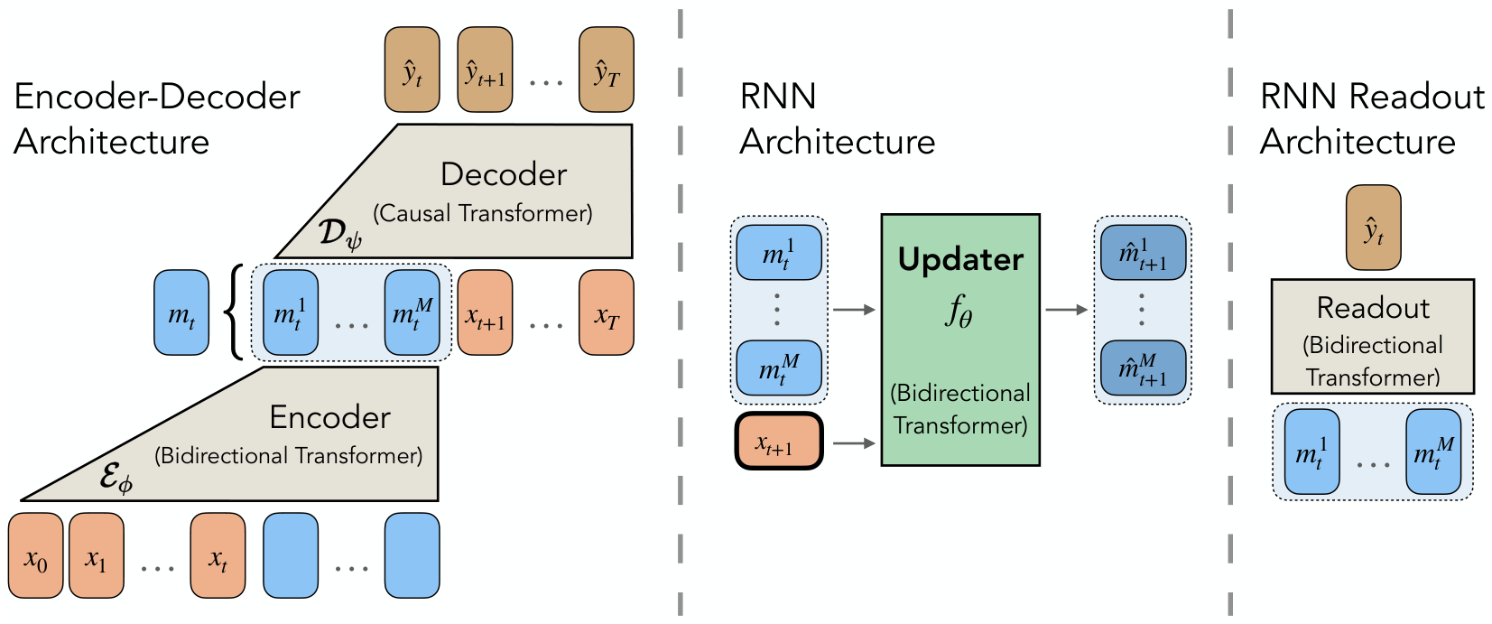
Our primary architecture used for most experiments is shown in Figure 15.
Encoder Architecture We use the same encoder model architecture across all experiments. The model begins with an embedding layer to embed input tokens, and a list of learned memory token registers. The input and register tokens are concatenated and processed by a stack of bidirectional (full attention mask) Transformer blocks. We use bidirectional model because the goal is to create a holistic representation of the entire input sequence. The register tokens are then interpreted as memory tokens at the output. Note that a single memory consists of a list of memory tokens,
Decoder Architecture We use the same decoder model architecture across all experiments. The decoder has an embedding layer to embed input tokens, which is weight shared with the encoder model. The memory tokens from the encoder and the embedded future input tokens are concatenated, and then processed by a stack of causally masked Transformer blocks. We use a causal mask because the goal is to learn a generative model of the output sequence. Within the each Transformer block, we use rotary position encodings
Transformer-based RNN Architecture The Transformer-based RNN is our primary RNN architecture and is used for most experiments. It begins with an embedding layer for the current timestep’s input token. The memory tokens are concatenated with the input token and then processed by a stack of bidirectional (full attention mask) Transformer blocks to produce the output memory tokens. We perform RMSNorm on the output memory tokens.
MLP-based RNN Architecture The MLP-based RNN flattens the list of memory tokens into a single vector, concatenates it with the input token embedding, and passes them through an MLP. At the output, the model then unflattens them to be a list of memory tokens again. We perform RMSNorm on the output memory tokens.
GRU-based RNN Architecture The GRU-based RNN processes the
RNN Readout Architecture We use the same readout model architecture for all RNNs. The readout architecture takes in the memory tokens and processes them through a stack of bidirectional (full attention mask) Transformer blocks Figure 15 shows the readout architecture.
B.2 Datasets
B.2.1 Synthetic Tasks
Retrieval to test Gradient Stability The retrieval task requires the model to remember and reproduce the token immediately following a designated identifier (token 0). For example, given
String Copy to test Memory Capacity The string copy task requires the model to reproduce a sequence in reverse order after a delimiter (token 0). For example, given
Stack Operations to test State Tracking The stack operations task requires the model to track the top element of a stack through a sequence of push and pop operations (denoted by token 0). For example, given
Keys and Values to test Associative Recall The keys and values task requires the model to store and retrieve associations between keys and values, then recall the value corresponding to a queried key
Modular Arithmetic to test In-Context Learning The modular arithmetic task requires the model to infer a latent linear rule from in-context examples and apply it to novel inputs
B.2.2 Natural Tasks
TinyStories TinyStories is a curated dataset of short stories generated by OpenAI’s
MNIST MNIST is a classic image dataset consisting of handwritten digits
Sketchy Sketchy is an image dataset of human-drawn sketches
B.3 Algorithms
For all experiments, we use the AdamW optimizer with a weight decay of 0.01 and learning rates tuned separately for each algorithm. For all methods, gradients are clipped to a maximum global norm of 1. Gradient clipping is expected to be particularly beneficial for BPTT.
After SMT, we transfer the decoder weights to the RNN readout module. During DMT, this readout head is further finetuned to optimize the next-token prediction loss using RNN-generated memory states. Importantly, this task loss updates only the readout head and not the RNN dynamics function, and therefore does not constitute temporal credit assignment for the RNN itself. Instead, finetuning serves to adapt the readout head to imperfections in the memory states generated by the RNN.
Synthetic Experiments We set
Other Experiments To evaluate the expectation in
By default for SMT, we set , , , ,
memory tokens. The encoder is 8 layers deep, while the decoder is 4 layers deep. The RNN is also 8 layers deep, and its readout function is 4 layers deep. We use a batch size of 128 sequences.
C Additional Experiments
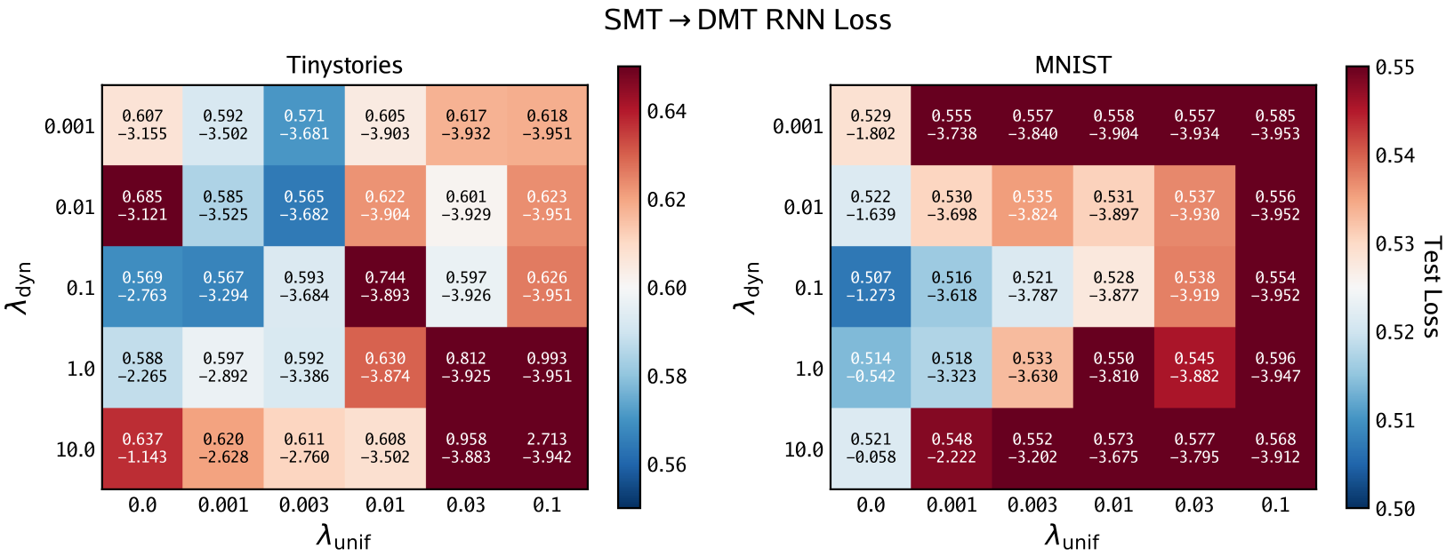
Figure 16 shows the results of ablating the
Figure 17 shows more samples of generations from Figure 4. Samples generated by the BPTT RNN (Transformer backbone) seem to only pick up on short range context and act accordingly: either output large streaks of white or black based on the current row. BPTT RNN (GRU backbone) improves this significantly, but still fails to capture the nuanced structure of digits. SMT→DMT RNN (Transformer backbone) is able to capture this structure quite well.
Figure 18 shows more samples of generations from Figure 5. These generations are often not fully interpretable, but do capture the stroke structure of human-drawn sketches. Capturing this stroke structure is itself a difficult problem, given the long-horizon nature of pixel sequence modeling.
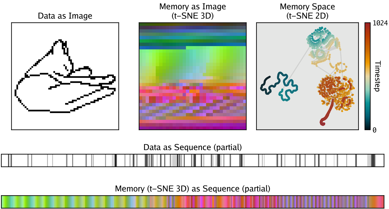
Figure 19 provides an analysis of our Sketchy RNN as it “reads” a sequence corresponding to the classic Attneave’s cat image
D Compute Resources Used
All individual training runs were conducted on one H200 GPU within 48 hours. The synthetic experiments comprised more than 375 small-scale training runs, while the real-data experiments required 144 large-scale runs.
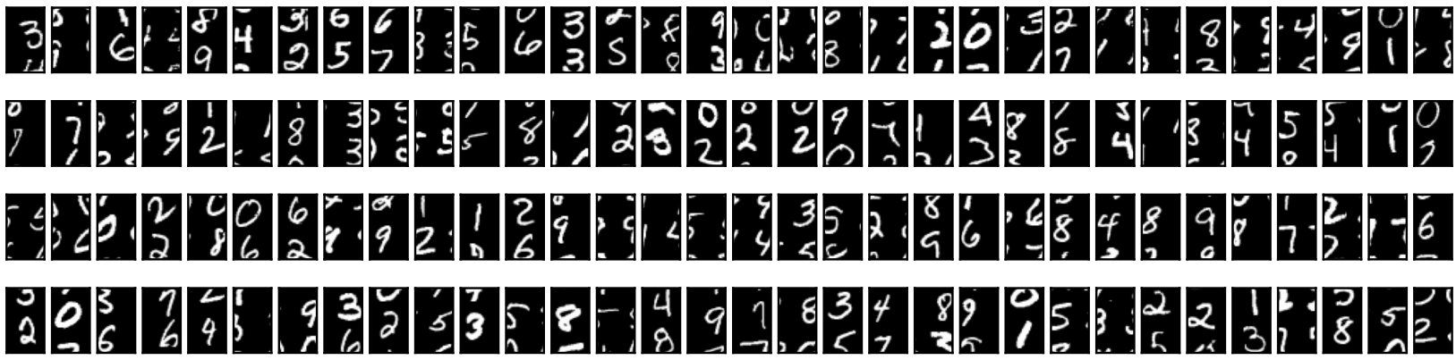
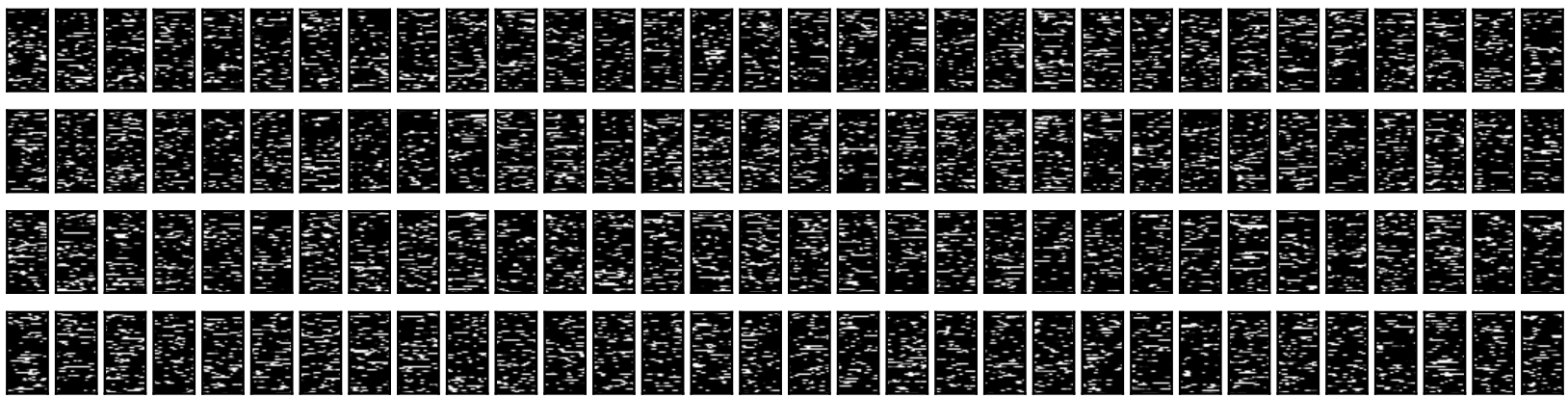
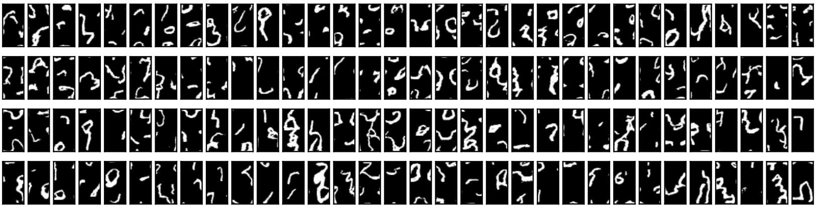
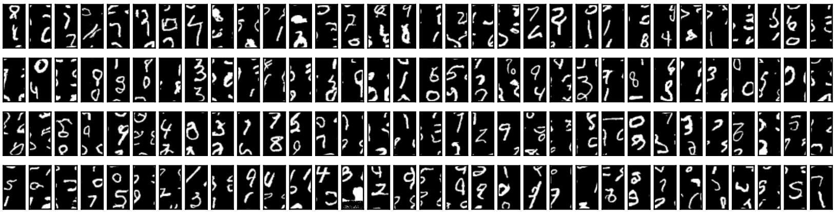
Figure 17: Additional MNIST Samples. Here we give more examples of samples of MNIST images generated by the various methods. SMT
E Sequence to Set Reframing
As described in Section 2.2, consider a hypothetical oracle memory-encoding model
Claim Let
with
Proof We construct
This is well-defined because the timestamps are distinct integers, so the sort order is unique. The resulting sequence is identical to the original
Moreover,
Since
Implication This result implies that any sufficiently expressive permutation-invariant set model can in principle exactly model a recurrent memory function. Because sets are unordered, time-parallel processing naturally follows. In particular, Transformer-based architectures can be interpreted as operating over sets of timestamped tokens rather than strictly ordered sequences.
Notably, the proof is constructive:
However, our empirical results suggest that even relatively shallow Transformer encoders can learn highly effective memory representations for both synthetic and natural tasks. Thus, despite lacking full theoretical expressivity, this sequence-to-set reframing may still provide a practical strategy for memory pretraining. For full expressivity, some light-weight post-training may be required.
F Encoder Markovian Training
SMT consists of two primary objectives: future predicting with
Claim Let and
with memory state
Proof By optimality of
Note that and , so optimality of at time implies it is also sufficient for given :
By optimality of , it is a minimal sufficient statistic of for predicting given . Minimality means retains no information from beyond what is predictively necessary. Since already constitutes a sufficient statistic for this same prediction task—as shown above—minimality of forces it to be a function of :
for some measurable . Therefore is determined entirely by , and conditioning on these renders it independent of all earlier context:
which is equivalent to . Hence is Markovian. ■
Implication This result establishes that under ideal conditions—sufficient encoder and decoder capacity, infinite future horizon, and exact optimization—the memory states learned by
In practice, finite capacity and approximate optimization relax this property, leaving with residual dependence on beyond . This gap motivates jointly training the dynamics loss alongside to explicitly encourage Markovian structure in the learned memory sequence.
Relatedly,