Topological constraints on self-organization in locally interacting systems

**PHILOSOPHICAL TRANSACTIONS A** [royalsocietypublishing.org/rsta](https://royalsocietypublishing.org/rsta)

Research
Cite this article: Sacco F, Sakthivadivel D, Levin M. 2026 Topological constraints on self-organization in locally interacting systems. Phil. Trans. R. Soc. A 384: 20250011. https://doi.org/10.1098/rsta.2025.0011

Received: 25 January 2025
Accepted: 8 August 2025

One contribution of 18 to a theme issue ‘World models in natural and artificial intelligence’.

Subject Areas:
statistical physics, complexity, artificial intelligence

Keywords:
phase transitions, potts model, self-organization, emergence, diverse intelligence

Author for correspondence:
Dalton Sakthivadivel
e-mail: dsakthivadivel@gc.cuny.edu

Francesco Sacco $^{1}$ , Dalton Sakthivadivel $^{2}$ and Michael Levin $^{1, 3}$

$^{1}$ Tufts University, Allen Discovery Center, Medford, MA, USA
$^{2}$ Department of Mathematics, CUNY Graduate Center, New York, NY, USA
$^{3}$ Tufts Center for Regenerative and Developmental Biology, Tufts University, Medford, MA, USA

DS, [0000-0002-7907-7611](); ML, [0000-0001-7292-8084]()

GRAY

All intelligence is collective intelligence, in the sense that it is made of parts that must align with respect to system-level goals. Understanding the dynamics that facilitate or limit navigation of problem spaces by aligned parts thus impacts many fields ranging across life sciences and engineering. To that end, consider a system on the vertices of a planar graph, with pairwise interactions prescribed by the edges of the graph. Such systems can sometimes exhibit long-range order, distinguishing one phase of macroscopic behaviour from another. In networks of interacting systems, we may view spontaneous ordering as a form of self-organization, modelling neural and basal forms of cognition. Here, we discuss necessary conditions on the topology of the graph for an ordered phase to exist, with an eye towards finding constraints on the ability of a system with local interactions to maintain an ordered target state. By studying the scaling of free energy under the formation of domain walls in three model systems—the Potts model, autoregressive models and hierarchical networks—we show how the combinatorics of interactions on a graph prevent or allow spontaneous ordering. As an application, we are able to analyse why multiscale systems like those prevalent in biology are capable of organizing into complex patterns, whereas rudimentary language models are challenged by long sequences of outputs.

This article is part of the theme issue ‘World models in natural and artificial intelligence’.

© 2026 The Authors. Published by the Royal Society under the terms of the Creative Commons Attribution License [http://creativecommons.org/licenses/by/4.0/](http://creativecommons.org/licenses/by/4.0/), which permits unrestricted use, provided the original author and source are credited.

1. Introduction

Self-organization is a fascinating phenomenon observed across diverse systems in nature and technology. In biology, self-organization of complex structures and functions, from subcellular machinery to multicellular morphogenesis, requires alignment of parts to navigate a problem space towards specific adaptive ends [1–7]. Dynamics of this form can be viewed as a sort of autopoietic cognition, raising interesting questions about how self-organizing systems navigate through configuration space given some target morphology [8–19]. More recently, current approaches to machine learning have involved physics-inspired models such as the Hopfield network [20–22] and spin glasses [23] and energy-based [24] or diffusion models [25]. In these systems, in order to maintain a pattern out of equilibrium or produce sensible data over long time spans, there must exist a ‘condensed’ phase with long-range order. While some systems—like those prevalent in biology—demonstrate remarkable abilities to organize at large scales, other systems that also exhibit some degree of collective intelligence—such as natural language models—have much more limited capabilities [26–30]. Despite this, spin systems have also been used to model cellular morphogenesis [31–35], suggesting the difference goes beyond the substrate of intelligence considered. This article is motivated by the following question: what is the functional distinction between simple language models and multicellular organisms, and can generative AI harness that property to achieve long-range order? In particular, we are interested in placing explicit thermodynamic bounds on the probability of some example systems occupying such a phase, with applications to estimating their capability to self-organize.

The question of how probable ordered configurations are as the number of elements increases is equivalent to asking about the existence of a phase transition, where the ultimate energetic constraints on the existence of an ordered phase arise from the topology of the interactions between subunits of the system. A quick argument due initially to Landau–Lifshitz [36]Landau and Lifshitz, §149 shows why the one-dimensional Ising model, the prototypical spin system, has no ordered phase at any temperature; their study of scaling is the technique we will use in this article, so we will review it here. Recall that a thermodynamically favourable change in state is one which decreases the free energy

Δ F = Δ E - T Δ S

delta F equals delta E minus T delta S

Suppose a domain wall of perimeter $P$ P forms at an arbitrary location in the chain. Using an effective Hamiltonian, calculating the free energy of the system with zero domain walls and the system with one domain wall shows that the change in free energy scales like $- T lo g P$ minus T log P, meaning that forming a domain wall is always thermodynamically favourable for sufficiently large $P$ P. As a result, long chains are unstable under thermal fluctuations, and disorder always propagates through the chain. In the thermodynamic limit, there is no spontaneous magnetization. Ising (1925)Ising proves this by finding the partition function and calculating the mean magnetization analytically in his celebrated 1925 paper, but the advantage of the argument of Landau and Lifshitz is that it applies generically to phase transitions in many different sorts of one-dimensional system (though the details prove somewhat subtle) and uses a simple scaling argument. The argument to the contrary in dimension greater than one is famously due to Peierls [37], where it is shown that the change in internal energy has a factor of $P$ P balancing the change in entropy. This is found by computing the number of spins an ‘island’ interacts with—which is highly dependent on the properties of the lattice.

The main results in this article concern when an ordered phase can exist in a self-organizing system based on its interactions. We will focus on the scaling relationship between energy and entropy as it is determined by combinatorial topology. We begin this section by presenting our argument for a large universality class of models and deriving the necessary conditions for the existence of an ordered phase in this class. In §3, we analyse the one-dimensional Potts chain as a simple model system, recovering the argument given by Landau–Lifshitz in a more general setting. §4 maps autoregressive models [38] onto this one-dimensional framework and proves their

A diagram showing a chain of variables labeled s sub minus one through s sub five. A box labeled H sub two groups the variables from s sub zero to s sub four. Figure 1. A local Hamiltonian in dimension one. The Hamiltonian of this chain is a sum of windowed Hamiltonians of length $ω = 5$ omega equals five. Pictured is the second window; the first begins at $s_{- 1}$ s sub minus one.

inability to maintain long-range order. A discussion of transformers follows in §5section five. In §6section six, we apply these results to multiscale systems to evaluate the possibility of order in that context, based on the hierarchies built into the topology of interaction. Finally, we discuss implications of these results and future directions in §§7 and 8sections seven and eight. We conclude that certain systems cannot remain ordered over long ranges for all time and suggest this no-go theorem as a source of fitness pressure for biological phenomena like stigmergy and embodiment. The key insight of our work will be that topology is the critical factor differentiating these systems. Namely, while cells in the human body can coordinate and organize over vast scales, forming coherent tissues and organs, language models struggle to maintain consistency beyond their limited context windows. This disparity stems directly from the underlying topology of interactions in these systems.

2. The main argument

Consider a $k$ k-vertex graph with $k$ -by- $k$ k by k adjacency matrix $G$ G and an $n$ n-ary variable on each vertex. Denote each such variable as $s_{i}$ s sub i, indexed by $i \in {1, \dots, k}$ i from one to k. The interactions between any set of spins will be given by the Hamiltonian $H$ H.

Definition 1. A windowed Hamiltonian $H$ H is a Hamiltonian in that spin–spin interactions are defined only within a finite window of interaction $ω$ omega.

Remark. Without loss of generality, we will assume that the lowest energy state of any windowed Hamiltonian is zero. We will moreover assume the existence of an upper bound to the highest energy of any possible window Hamiltonian, $E_{i}^{max} ⩽ E^{max}$ E max sub i is less than or equal to E max.
We call a sum of such effective Hamiltonians a local Hamiltonian. In particular,

Definition 2. A local Hamiltonian is a Hamiltonian which can be decomposed into a sum of several window Hamiltonians $H = \sum_{u} H_{u}$ H equals the sum over u of H sub u, all of which have the same window length $ω$ omega.

See figure 1 for a depiction. For the purpose of intuition, one may notice a local Hamiltonian with window size equal to one is a discrete Markov field.

Our methodology will be given by the following prescription:

Begin with the system in one of the ordered configurations, e.g. one of the stored patterns
Create a domain wall
Estimate the energy gained by the system
Find the asymptotics of the free energy as the number of domain walls increases

Computing the change in $F$ F by changing the number of domain walls requires detailed knowledge of the combinatorics of the interactions on the graph. Instead, we can use the structure imposed by the windows. Namely, we have regulated the length of interactions such that we need only count the number of windows containing a domain wall. This does away with the particularities of the lattice and so can be applied to systems on very generic graphs. We will explore this in the present section.

The most general way to consider the interaction between the elements of our system is if the interactions are represented by a graph Hamiltonian. For simplicity, we will assume that the

Two diagrams comparing a graph G and a graph Hamiltonian H. On the left, graph G shows six vertices s1 through s6 connected in a circular pattern with two cross-connections. On the right, graph H shows the same structure but with edges labeled e1 through e7 representing coupling strengths. Figure 2. Illustration of a graph Hamiltonian. Left: the graph $G$ G represents the adjacency matrix of an undirected graph with six vertices, where edges indicate connections between vertices $s_{i}$ s sub i. Right: the graph $H$ H represents the graph Hamiltonian, where the coupling strengths $e_{i}$ e sub i have come from $\overset{ˉ}{H}$ H bar.

edges of the graph are fixed in time; one can easily justify this by appealing to an adiabatic approximation where the birth or death of edges is unlikely for the timescale on which observations are made.

Definition 3. Let $G$ G be the adjacency matrix of a graph on $k$ k vertices and $\overset{ˉ}{H}$ H bar a $k$ -by- $k$ matrix. A graph Hamiltonian is the Hamiltonian of a weighted directed graph; namely, a Hamiltonian which can be written as

H = \overset{ˉ}{H} ⊙ G

H equals H bar entry-wise product G

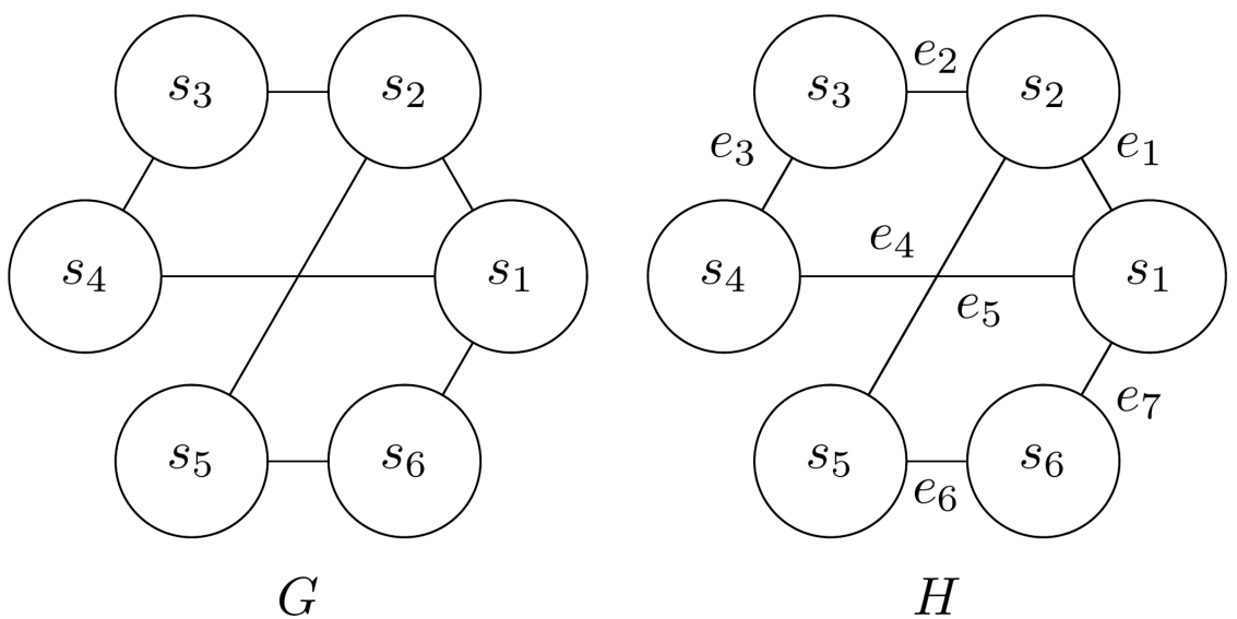
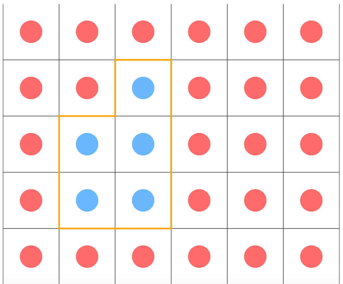
where $⊙$ the symbol is entry-wise multiplication and $\overset{ˉ}{H}$ H bar has as entries the coupling strengths of the system.

See figure 2. We will now give a recipe for computing the scaling behaviour of energy and entropy for a graph Hamiltonian system. For the sake of simplicity, we will work with square planar embeddings of graphs (grid-like lattices) in this article. In these cases, a domain wall and its perimeter can be easily defined (figure 3).

Let $H$ H be a graph Hamiltonian and $P$ P be the perimeter length of a domain wall. As the perimeter length increases, the number of possible configurations of domain barriers increases, increasing the entropy of the system $Δ S$ delta S. We say that the entropy gained scales as $f_{S}$ if

Δ S = O (f_{S} (P)) .

delta S is of order f S of P

We give a similar definition for energy scaling: as the perimeter length increases, the upper and lower bounds of the energy gained scale as $O (f_{E}^{high} (P))$ and $O (f_{E}^{low} (P))$ order f E high of P and order f E low of P, respectively. If $f_{E}^{high} = f_{E}^{low} \equiv f_{E}$ f E high equals f E low, defined as f E we say that the energy gained scales as $f_{E}$ , that is, $Δ E = O (f_{E} (P))$ delta E is of order f E of P.

If we can estimate how the energy and entropy scale, we can verify the existence or non-existence of an ordered phase without knowing the exact formulae for $E (P)$ and $S (P)$ E of P and S of P, only considering how they scale as $P \to \infty$ P goes to infinity.

Proposition 1. If $O (f_{S}) = O (f_{E})$ then there exists an ordered phase.

Proof. Suppose $O (f) = O (f_{S}) = O (f_{E})$ . Then the change in free energy is

Δ F = Δ E - T Δ S = P \to \infty lim O (f (P)) - T O (f (P)) .

............................................................................................................. Downloaded from [Royal Society Publishing](http://royalsocietypublishing.org/rsta/article-pdf/doi/10.1098/rsta.2025.0011/6138032/rsta.2025.0011.pdf) by guest on 05 July 2026

A 5 by 5 grid of circles, with most being red and a small cluster of five being blue. An orange line outlines the boundary between the blue and red regions. Figure 3. Two different domains in a two-dimensional grid. The perimeter that separates the two domains is drawn in orange.

If we now take $T$ T to zero, the change in free energy becomes increasingly positive. As such, the creation of a domain wall is unfavourable. ■

In this way, we can rule out details of the system that could complicate the combinatorics—for example, the number of stored patterns. Let

\pi = (\dots, s_{-1}, s_0, s_1, \dots) $$<yap-speak>pi equals the sequence s sub i</yap-speak> denote a ground state of the system. One may think of this state as a stored pattern or morphogenetic configuration. When there is a ground state degeneracy—that is, multiple states with zero energy exist, for instance, if a Hopfield model has $m > 1$<yap-speak>m greater than one</yap-speak> stored patterns—they will be enumerated as

\pi^\alpha = (\dots, s_{-1}^\alpha, s_0^\alpha, s_1^\alpha, \dots), \quad 1 < \alpha \leqslant m.

We can show that the number of such patterns affects neither the scaling of the entropy nor energy. **Lemma 1.** Let $H = \sum_u H_u$<yap-speak>H equal the sum over u of H sub u</yap-speak>. If there exist two energies $E^{\text{max}}, E^{\text{min}}$<yap-speak>E max and E min</yap-speak> which are the greatest and least non-zero energy levels of all the windowed Hamiltonians $H_u$<yap-speak>H sub u</yap-speak>, respectively, then at thermal equilibrium, the ability to converge to an ordered phase is independent of energy levels and window sizes. *Proof.* For any $H_u$<yap-speak>H sub u</yap-speak> let $\omega_1$<yap-speak>omega one</yap-speak> be the size of the smallest window and $\omega_2$<yap-speak>omega two</yap-speak> that of the largest. The energy gained from the creation of a domain wall is bounded by

\omega_1 P E^{\text{min}} \leqslant \Delta E \leqslant \omega_2 P E^{\text{max}}.

In both cases, we have $E = O(P)$<yap-speak>E is of order P</yap-speak> so that the asymptotics of the system depend only on the perimeter length. ■ **Lemma 2.** Let $H$<yap-speak>H</yap-speak> be a graph Hamiltonian with $m > 1$<yap-speak>m greater than one</yap-speak> stored patterns. At thermal equilibrium, the ability to converge to an ordered phase is independent of $m$<yap-speak>m</yap-speak>. <yap-show> Downloaded from [royalsocietypublishing.org](http://royalsocietypublishing.org/rsta/article-pdf/doi/10.1098/rsta.2025.0011/6138032/rsta.2025.0011.pdf) by guest on 05 July 2026 </yap-show> *Proof.* Let $B(P)$<yap-speak>B of P</yap-speak> be the number of possible configurations of domain barriers with perimeter $P$<yap-speak>P</yap-speak>. The change in entropy due to the creation of a domain barrier can always be written as

\Delta S = \log [(m - 1)B(P)] = \log B(P) + \log(m - 1).

<yap-speak>delta S equals the log of m minus one times B of P, which is the log of B of P plus the log of m minus one.</yap-speak> In the thermodynamic limit, the term proportional to the number of barriers increases, while the term proportional to the number of patterns stored stays constant. As such, its contribution can be ignored. ■ Since neither the shape nor number of stored patterns affects the thermodynamics of the problem, and neither does the size of the interaction window, we reduce our analysis to the nearest-neighbour Ising model. Our main technical result is the following topological equivalence theorem: **Theorem 1.** *All local Hamiltonians on lattices with the same combinatorial structure have asymptotically equivalent free energies.* *Proof.* We will show that we can approximate any $H$<yap-speak>H</yap-speak> with the Hamiltonian of some arbitrary other model in such a way that their asymptotics are equivalent, implying that in the thermodynamic limit, the Peierls argument depends only on the perimeter length in the approximate system. Let $H = \sum_u H_u$<yap-speak>H equals the sum over u of H sub u</yap-speak> be a local Hamiltonian on a planar graph $G$<yap-speak>G</yap-speak> with any spin $i$<yap-speak>i</yap-speak> coupled to $\eta_i$<yap-speak>eta sub i</yap-speak> other spins. Let $H_0$<yap-speak>H zero</yap-speak> be the Hamiltonian of an arbitrary system. One knows by the Bogoliubov inequality <yap-show>[39]</yap-show> that

F \le F_0 + \langle H - H_0 \rangle_0

<yap-speak>F is less than or equal to F zero plus the expectation of H minus H zero with respect to the H zero ensemble</yap-speak> and therefore that if $H$<yap-speak>H</yap-speak> and $H_0$<yap-speak>H zero</yap-speak> are asymptotically equivalent then $F \sim F_0$<yap-speak>F is asymptotic to F zero</yap-speak>. As the perimeter length increases, we have $E = O(P)$<yap-speak>E is order P</yap-speak> and $E_0 = O(P_0)$<yap-speak>E zero is order P zero</yap-speak> by Lemma 1. If the combinatorics of the lattices are the same—namely, if the set of $\eta_i$<yap-speak>eta sub i</yap-speak> is equal on both lattices—then we can take $P = P_0$<yap-speak>P equals P zero</yap-speak>. The change in the energy is computed by the Hamiltonian of the new configuration, implying $H - H_0 \sim 0$<yap-speak>H minus H zero is approximately zero</yap-speak>. By Lemma 2, the probability of any disorder occurring is asymptotically the same in both systems, so that the *change* in free energies is also asymptotically equivalent. The claim follows. ■ **Corollary 1.** *The capacity for self-organization in any system on a graph $G$<yap-speak>G</yap-speak>—that is, the existence or non-existence of a phase transition—is equivalent to that of a nearest-neighbour Ising model on the same graph, with*

H_0 = -J \sum_{i,j} s_i s_j

< y a p - s p e ak > H z er oe q u a l s min u s J t im es t h es u m o v er ian d j o f ss u bi t im esss u bj < / y a p - s p e ak > * an d tw os t or e d p a tt er n s *

\begin{align} \pi^1 &= (1, 1, 1, \dots, 1) \ \pi^2 &= (-1, -1, -1, \dots, -1). \end{align}

<yap-speak>pi one as a vector of ones and pi two as a vector of minus ones</yap-speak> An important remark is that we do not claim the phase transitions are the same. Naturally, they will differ in general, for instance, if there are more stored patterns in one system than the other. It is the existence of a phase transition from the topology of the lattice that we study. ## 3. Stored patterns in the windowed With this in hand, we can study our first model system: the one-dimensional Potts model. The Potts model is a variant of the Ising model whose state vectors are richer than simply binary numbers. In particular, one can encode data in a Potts chain by choosing different spin configurations, <yap-show> Downloaded from [Royal Society Publishing](http://royalsocietypublishing.org/rsta/article-pdf/doi/10.1098/rsta.2025.0011/6138032/rsta.2025.0011.pdf) </yap-show> recalling the discussion in the Introduction. It is a suitable model to describe stored images or other configurations of multiply-valued variables. **Definition 4.** Let $n$<yap-speak>n</yap-speak> be a finite positive number. A Potts chain $\mathcal{C}$<yap-speak>C</yap-speak> is a $\mathbb{Z}$-indexed set of $n$-ary integer symbols; that is, a chain of spins $s_i$<yap-speak>s sub i</yap-speak> indexed by $i \in \mathbb{Z}$<yap-speak>i in the set of integers</yap-speak>, where each $s_i$<yap-speak>s sub i</yap-speak> can assume any integer value in $\{1, \dots, n\}$. It follows from Theorem 1 that it is sufficient to consider the scaling of $\mathcal{C}$<yap-speak>C</yap-speak> to establish the existence of an ordered phase. In the same fashion as Landau–Lifshitz, it can be shown that local Hamiltonians in dimension one do not converge to a prescribed ordered state, since the formation of a domain wall always 'interrupt' the pattern. **Theorem 2.** *Let $H$<yap-speak>H</yap-speak> be a one-dimensional local Hamiltonian with $m > 1$<yap-speak>m greater than one</yap-speak> stored patterns. At non-zero temperature, the formation of a domain wall is thermodynamically favourable.* *Proof.* Suppose that our Potts chain starts out in the first ground state or pattern, $\mathcal{C} = \pi^1$<yap-speak>C equals pi one</yap-speak>. If

\Delta F = \Delta E - T \Delta S < 0,

<yap-speak>the change in free energy, delta F, equals delta E minus T delta S, which is less than zero</yap-speak> so that the free energy of the system decreases upon the formation of a domain barrier, then the formation of a domain barrier is thermodynamically favourable. It is immediate that any $\pi^\alpha$<yap-speak>pi alpha</yap-speak> differs from some other $\pi^\gamma$<yap-speak>pi gamma</yap-speak> by at least one change in spin. In a sequence of length $L$<yap-speak>L</yap-speak> there are $L - 1$<yap-speak>L minus one</yap-speak> possible places where a domain wall can appear, and at each such place, we may obtain one of the $m - 1$<yap-speak>m minus one</yap-speak> other patterns saved. As such, the change in entropy of the system is

\Delta S = \log[(m - 1)(L - 1)].

<yap-speak>delta S equals the log of, m minus one times L minus one</yap-speak> Upon the formation of a domain barrier, the windowed Hamiltonians that intersect it will have non-zero, positive energy. By assumption, the energy is bounded, and no more than $\omega$<yap-speak>omega</yap-speak> windows can be affected by a domain wall, from which we obtain

0 \leqslant \Delta E \leqslant \omega E^{\text{max}}.

< y a p - s p e ak > z er o i s l ess t han or e q u a l t o d e l t a E, w hi c hi s l ess t han or e q u a l t oo m e g a t im es E ma x < / y a p - s p e ak > T h ec han g e in f r eee n er g y i s

\Delta F \leqslant \omega E^{\text{max}} - T \log[(m - 1)(L - 1)].

<yap-speak>delta F is less than or equal to omega E max minus T log of, m minus one times L minus one</yap-speak> Assume $T > 0$<yap-speak>T is greater than zero</yap-speak>. As $L$<yap-speak>L</yap-speak> increases, the right-hand side of the equation eventually becomes negative. ■ ## 4. Autoregressive models We begin this section by recalling in figure 4 the motivation stated in the introduction: contrasting the generation of textual features with the generation of morphological features, we would like to understand how the self-organizing nature of text is constrained by the topology of the interactions between subunits generating that text. We will now discuss a similar result as the one in the previous subsection, for autoregressive models. An autoregressive model is formed when values of a sequence are regressed against previous values of that sequence. Here, it will be defined as an estimator of some conditional probability distribution; namely, that of a sequence of observations of some data at step $i$<yap-speak>i</yap-speak>, given a history of observations until $i - 1$<yap-speak>i minus one</yap-speak>. **Definition 5.** Let $\{s_1, \dots, s_{i-1}\}$<yap-speak>the set s one through s i minus one</yap-speak> be a random $n$-ary sequence of length $i - 1$<yap-speak>i minus one</yap-speak>. Given a window (also called context) of length $\omega$<yap-speak>omega</yap-speak>, an order $\omega$<yap-speak>omega</yap-speak> autoregressive model computes

P(s_i \mid s_{i-1}, \dots, s_{i-\omega})

<yap-speak>the probability of s i given the sequence from s i minus one to s i minus omega</yap-speak> as a probability vector over $\{1, \dots, n\}$ by generating samples of $s_i$<yap-speak>s i</yap-speak> according to some random process on window states. Such a function is called an AR($\omega$<yap-speak>omega</yap-speak>) model in particular. As shorthand, we will denote the estimator whose output is $v$<yap-speak>v</yap-speak> when given a sequence $\{s_{i-1}, \dots, s_{i-\omega}\}$<yap-speak>s sub i minus one through s sub i minus omega</yap-speak> as $M$<yap-speak>M</yap-speak>:

v := M(s_i \mid s_{i-1}, \dots, s_{i-\omega}).

The function $M$<yap-speak>M</yap-speak> has the type of a conditional probability distribution. We further write

P(s_i = c) = M(s_i = c \mid s_{i-1}, \dots, s_{i-\omega})

for the $c$-th component of $v$<yap-speak>v</yap-speak>. Conceptually, we have the picture in figure 5. To fit this in the discussion of patterns and long-range order in spin chains, we find the following theorem useful. We will set the convention that if $u - \omega < 1$<yap-speak>u minus omega is less than one</yap-speak> then the window is empty at that index, and that conditioning on the empty set is the same as taking unconditional probability. **Theorem 3.** *A unique local Hamiltonian with window length $\omega$<yap-speak>omega</yap-speak> can be associated to any AR($\omega$<yap-speak>omega</yap-speak>) model.* *Proof.* Let $M$<yap-speak>M</yap-speak> be our autoregressive model, and $s_{i-1}, \dots, s_{i-\omega}$<yap-speak>s sub i minus one through s sub i minus omega</yap-speak> our input sequence. The probability that the next observed spin in the sequence is equal to $c$<yap-speak>c</yap-speak> is

P(s_i = c) = M(s_i = c \mid s_{i-1}, \dots, s_{i-\omega}).

Suppose[^1] we assign an energy to each possible $c$<yap-speak>c</yap-speak> with a scalar function $E : \{1, \dots, n\} \to \mathbb{R}$<yap-speak>E from the set one to n into the real numbers</yap-speak> and constant weight $\beta \geqslant 0$<yap-speak>beta greater than or equal to zero</yap-speak>, such that

\beta E_c = -\log P(s_i = c) + \text{const.} \quad \text{with} \quad c \in {1 \dots n}.

S e tt h eco n s t an t in s u c ha w a y t ha tt h e l o w es t e n er g y s t a t e ha se n er g y e q u a l t oz er o . N o w d e f in e a w in d o w e d H ami l t o nian

H_u(s_u) = -\log M(s_u \mid s_{u-1}, \dots, s_{u-\omega}) + \text{const}

for any $u$<yap-speak>u</yap-speak> in $\{1, \dots, i\}$<yap-speak>the set one to i</yap-speak> so that the probability of any $u$th token occurring before $i$<yap-speak>i</yap-speak> is conditioned on the window preceding it. The full local Hamiltonian is the sum

H = \sum_u H_u(s_u)

in an obvious way. ■ *Remark.* By Theorem 3, the generation of samples by an autoregressive model can now be seen as sampling from a Boltzmann distribution over sequences. We close this subsection with the following conclusion. The free energy can be calculated by $F = E - \beta^{-1}S$<yap-speak>F equals E minus beta inverse S</yap-speak> as usual. By Theorem 3, autoregressive models are one-dimensional systems described by a local Hamiltonian. The following corollary is then a consequence of the scaling argument in Theorem 2. **Corollary 2.** *For any finite $\beta$<yap-speak>beta</yap-speak>, an autoregressive model is unable to converge to a single stored pattern.* ## 5. Transformers and attention An interesting question to ask is what these results imply for the organizational capabilities, and hence intelligence, of large language models. Most state-of-the-art language models of today are [^1]: One could appeal to Gibbs’ equation or more general maximum entropy principles to do so. decoder-only transformer architectures <yap-show>(see [40])</yap-show>, meaning that to predict the next word (or token) they perform autoregression on all the previous elements of text—in other words, they are autoregressive at inference time. Indeed, transformers can be described as spin collectives <yap-show>[41–43]</yap-show>, with training dynamics under asynchronous updates behaving like a spin chain evolving under Glauber dynamics and text generation being sampling from the corresponding equilibrium distribution, just as we have modelled autoregression by a spin chain here. A consequence of the results in §4 is a fundamental limitation on the coherence of a simple version of a large language model for long sequences of outputs—and hence an explanation for limitations observed in papers such as <yap-show>[30]</yap-show>. **Proposition 2.** *Causally masked attention in a decoder-only model has no ordered phase.* *Proof.* Let $s \in \mathbb{R}^k$<yap-speak>s in R to the k</yap-speak> be the configuration of the network, $X$ a matrix of $m$ stored patterns $(\pi^1, \dots, \pi^m)$ with any $(X)_\alpha = \pi^\alpha = (s_1, \dots, s_k)$ and $X_{i\alpha} = \pi_i^\alpha = s_i$, and $\beta$<yap-speak>beta</yap-speak> a constant scalar. Now $X$ is a $k$-by-$m$ matrix of $n$-ary variables. One knows <yap-show>(see [41])</yap-show> the standard attention algorithm with the identity matrix for weights is a modern Hopfield network with an exponential potential function <yap-show>[22]</yap-show>. The asynchronous updates maximize the probability of a Gibbs distribution, where the energy $\beta E(s)$ of a configuration, $-\log P(s) + \text{const}$, is

-\log \left( \sum_{\alpha=1}^m \exp \left( \beta \sum_{i=1}^k X_{i\alpha} s_i \right) \right) + \frac{\beta}{2} \sum_{i=1}^k s_i s_i + \log m + \frac{\beta}{2} \left( \max_\alpha |X_\alpha| \right)^2.

With a causally-masked positional encoding from $i - \omega$ to $i$, the expression at $i$ with context length $\omega$<yap-speak>omega</yap-speak> becomes

-\log \left( \sum_{\alpha=1}^m \exp \left( \beta \sum_{j=i-\omega}^i X_{j\alpha} s_j \right) \right) + \frac{\beta}{2} \sum_{j=i-\omega}^i s_j s_j + \log m + \frac{\beta}{2} \left( \max_\alpha |X_\alpha| \right)^2.

This can easily be seen as an expression for a local Hamiltonian in a particular $\text{AR}(\omega)$<yap-speak>A R omega</yap-speak> model; it follows from Theorem 3 that we can apply Theorem 2 to the transformer, completing the proof of the statement. ■ For simplicity, we have used no mapping in an associative space; however, the result generalizes readily to those cases by the results in <yap-show>[41]</yap-show>. More sophisticated large language models employ multi-headed attention algorithms <yap-show>[44]</yap-show>, where different attention heads in the decoder are attenuated to different classes of relationship. However, even in attention with heads for long-range dependencies, a maximum context length is imposed as a hyperparameter for reasons of computational cost <yap-show>(see the implementations in the review [45])</yap-show>. While the algorithm itself is more sophisticated and allows better performance when applied to two-dimensional data (e.g. images), the coherence of a sequence of text is constrained by context length, which is a realistic and necessary-to-consider constraint given hardware. More discussion on this will be given at the end of §6. ## 6. Large hierarchical systems on graphs In many systems of interest, there are hierarchical interactions, i.e. effective interactions between subgraphs. Many multiscale systems in biology and physics exhibit complex patterns consisting of pockets of regularity assembled into structures with global irregularity, such as tissues with different morphogenetic features assembled out of their constituent cells <yap-show>[46–51]</yap-show>, functional networks in the brain consisting of regions specialized to process certain sorts of information <yap-show>[52–55]</yap-show>, and self-assembling molecules in active matter situations <yap-show>[56–60]</yap-show>. In this section, we will investigate the interplay between the scaling of free energy at one level of a hierarchy and that of another, <yap-show> Downloaded from http://royalsocietypublishing.org/rsta/article-pdf/doi/10.1098/rsta.2025.0011/6138032/rsta.2025.0011.pdf by guest on 05 July 2026 </yap-show> ![Diagram illustrating the analogy between text generation and morphogenesis, showing navigation in morphological space, error correction, and regeneration.](./topological-constraints-on-self-organization-in-locally-interacting-systems-4.png)<yap-cap>**Figure 4.** Text generation in analogy to a morphogenetic process.</yap-cap> when the topology of the graph organizes those levels meaningfully, to quantify when such patterns are possible. We will complement the results in previous sections by showing that systems lacking hierarchical structure may be limited in their ability to form complex patterns. Recall that a clique is a (non-empty) complete induced subgraph (figure 6). Suppose there exist $\ell > 1$<yap-speak>ell greater than one</yap-speak> independent[^2] cliques in $G$<yap-speak>G</yap-speak>, with $n_1, \dots, n_\ell$<yap-speak>n one through n ell</yap-speak> vertices, respectively, and each $n_i > 2$<yap-speak>n i greater than two</yap-speak>. There will be a macrostate associated with each clique giving the magnetization of that subgraph. We will argue that there are ways for local order but global disorder to exist in systems with cliques. Since the effective behaviour of the system, i.e. the properties of the cliques, is often a meaningful experimental variable (and hence a useful macrostate), this means organizing a system hierarchically can create interesting order phenomena. In particular, we want to show that there can exist ‘hierarchical behaviours’, where each clique individually is a coherent phase, but that phase varies from clique to clique. [^2]: By independent, we mean the vertex set of each clique is disjoint from that of each other clique. For brevity, and without loss of generality[^3], we will assume the coupling constants $J$<yap-speak>J</yap-speak> are uniform across the graph. We will need the following observation before we prove our main theorem in this section. Recall that Boltzmann’s formula $S = k \log W$<yap-speak>S equals k log W</yap-speak> denotes by $W$<yap-speak>W</yap-speak> the multiplicity of a macrostate. A clique is positively (negatively) magnetized if all spins in the clique have value $+1$<yap-speak>plus one</yap-speak> ($-1$<yap-speak>minus one</yap-speak>). We will begin with $\ell$<yap-speak>ell</yap-speak> positively magnetized cliques. If the number (denote it $r$<yap-speak>r</yap-speak>) of ‘flipped’ (i.e. uniformly changed) cliques is a macrostate, then the multiplicity is the number of ways to arrange $r$<yap-speak>r</yap-speak> distinguished cliques out of the total $\ell$<yap-speak>ell</yap-speak> cliques. As such, we have

S = k \log \binom{\ell}{r}.

<yap-speak>S equals k times the log of ell choose r</yap-speak> **Theorem 4.** *Take any of the $\ell$<yap-speak>ell</yap-speak> cliques. There exist parameter regimes where individual cliques may change from positive to negative magnetization. For that temperature, take any individual $n_i$<yap-speak>n sub i</yap-speak>-clique and consider a spin within it. If the coupling of every spin in the clique is greater than $\frac{T}{2} \log n_i$ then the clique remains uniformly magnetized.* *Proof.* Flipping $r$<yap-speak>r</yap-speak> cliques from positive to negative magnetization takes an energy of $\sum_{\gamma=1}^{r} 2Jn_{i_\gamma}$, where $\gamma$<yap-speak>gamma</yap-speak> indexes cliques flipped, and has an entropy of the logarithm of $\ell$<yap-speak>ell</yap-speak> choose $r$<yap-speak>r</yap-speak>. The full change in free energy is

\Delta F = \sum_{\gamma=1}^{r} 2Jn_{i_\gamma} - T \log \frac{\ell!}{r!(\ell - r)!}

<yap-speak>the change in free energy delta F equals the sum from gamma equals one to r of two J n sub i gamma, minus T log of the combination formula ell factorial over r factorial times ell minus r factorial</yap-speak> so that the scaling behaviour of $r$<yap-speak>r</yap-speak> flips to

\Delta F \sim O(r) - TO(r \log \ell - r \log r + r),

where we have obtained the approximation of the entropy from $\binom{\ell}{r} \approx \ell^r / r!$ and Stirling’s formula. Clearly, if (up to some constant)

T > \frac{1}{\log \ell - \log r + 1}

then $\Delta F < 0$<yap-speak>delta F is less than zero</yap-speak>. Hence, there exist temperatures for which it is favourable for some number $r$<yap-speak>r</yap-speak> of entire cliques to change. Fix such a $T$<yap-speak>T</yap-speak>. Within an $n_i$<yap-speak>n sub i</yap-speak>-clique, there are $n_i$<yap-speak>n sub i</yap-speak> ways to flip a single spin. This takes energy $2J$<yap-speak>two J</yap-speak>. If we have $2J > T \log n_i$, then there is no domain wall within the clique. By minding constants in the $O(r)$ terms above, we show the hypothesis can be attained—namely, that there exist values of $T$<yap-speak>T</yap-speak> for which the inequality is satisfied. **Proposition 3.** *Let $n_{\text{max}}$<yap-speak>n max</yap-speak> be an integer greater than zero denoting the number of vertices in the largest clique. There exists a non-empty critical temperature range of hierarchical behaviour.* *Proof.* From the theorem above, we have

\frac{2J}{\log n_i} > T > \frac{2J \sum_{\gamma=1}^r n_{i_\gamma}}{r \log \ell - r \log r + r}.

< y a p - s p e ak > tw o J o v er l o g n s u bii s g r e a t er t han T, w hi c hi s g r e a t er t han tw o J t im es t h es u m o f n s u bi g amma, d i v i d e d b y r l o g e l l min u sr l o g r pl u sr < / y a p - s p e ak > W e a l so k n o w t ha t

rn_{\text{max}} \geqslant \sum_{\gamma=1}^r n_{i_\gamma}

<yap-speak>r times n max is greater than or equal to the sum of n sub i gamma</yap-speak> [^3]: This is because the $J$<yap-speak>J</yap-speak>’s do not affect the combinatorics used to compute the entropy; as in Lemma 1, we are permitted to simply take $J$<yap-speak>J</yap-speak> large enough to bound all of the true couplings in the clique. ![Diagram showing a sequence of tokens from s one to s thirteen with arrows indicating autoregressive dependencies.](./topological-constraints-on-self-organization-in-locally-interacting-systems-5.png)<yap-cap>Figure 5. An autoregressive model with $\omega = 5$<yap-speak>omega equals five</yap-speak>.</yap-cap> and

\frac{1}{\log n_i} \geqslant \frac{1}{\log n_{\max}},

so i t s u f f i ces t o t ak e

\frac{2J}{\log n_{\max}} > T > \frac{2Jrn_{\max}}{r\log \ell - r\log r + r}.

I t f o l l o w s t ha t

\frac{1}{\log n_{\max}} > T > \frac{1}{\log \ell - \log r + 1} n_{\max}.

Since the upper bound is a strictly decreasing function of $n_{\max}$<yap-speak>n max</yap-speak> with a singularity at one, and the lower bound is a linear function of $n_{\max}$<yap-speak>n max</yap-speak>, they intersect for some sufficiently small slope, before which the inequality is satisfied. We conclude that there exist $\ell, r$<yap-speak>ell and r</yap-speak> for which the set of satisfactory $T$<yap-speak>T</yap-speak> is non-empty. In particular, this occurs whenever

\frac{\ell}{r} > \frac{n_{\max}^{n_{\max}}}{e}.

Graph View

TTS

Topological constraints on self-organization in locally interacting systems

1. Introduction

2. The main argument