Neural Ordinary Differential Equations - Paper

year: 2018
paper: https://arxiv.org/abs/1806.07366
website: Steve Brunton🐐 Yannik Paper Explained
code: https://github.com/llSourcell/Neural_Differential_Equations/blob/master/Neural_Ordinary_Differential_Equations.ipynb nice example code!
connections: optimization, lagrange multiplier

---

overview and intuition

A ResNet can be thought of as a discrete-time analogs to an ODE:

$$h_{t+1}=h_t+f(h_t,{\theta }_t)$$

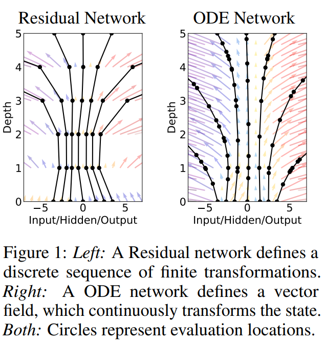
You update the representation in discrete steps layer by layer. Neural ODE views this as an infinite process with continous time.

The regular NN has a discrete gradient field, whereas the gradient field of the ODE Network is continous. The black dots are data points.

Again, with resnet you only model the distance (residual) of

$$x_{k+1}=x_k+\underset{\text{residual}}{\underbrace{f(x_k)}}$$

… this is a textbook euler numerical integrator (However euler integration, esp. with large time steps is a bad numerical integration method). So the resnet is doing euler integration over a vector field $f$, so what the neural network is learning, $x$, can also be thought of as a vector field, a differential equation $\dot{x}=f$

With NODE, we model the differential equation itself, instead of just a one-timestep-update or flow-map of the differential equation.

$$\frac{d}{dt}x=f(x)$$

So it is a generalization of resnets to continuous time, where you also use a fancier integrator and smallar or arbitrary time-steps to model the vector field very accurately.
The mathematician’s solution to this would be:

$$x_{k+1}=x_k{\int }_{t_k}^{t_{k+1}}f(x(\tau ))d\tau$$

That’s hard to compute, hence we approximate it (and you can use any integrator for that).

---

Classic dynamical system:

$$\dot{x}=f(x)⟹x(t_0+\Delta )=\underset{\text{flow map, }\varphi }{\underbrace{x(t_0)+{\int }_{t_0}^{t_0+\Delta t}d\tau }}$$

With NODE, $f$ is parametrized by a neural network

$$\dot{x}(t)=\underset{\text{neural net}}{\underbrace{f_{\theta }(x(t),t)}}⟹x(\tau )=\underset{\text{used in loss function, }\mathcal{L}}{\underbrace{\Phi (x(t_0),t_0,\tau ;\theta )}}$$

Free parameters:
$f_{\theta }\dots$ network parameters
$t_0\dots$ initial condition
$\Delta t\dots$ timestep

Hidden state: $x(\tau )$
… data is samples at discrete points in time (doesn’t need to be uniformly in time), so between any two data / measurement points, there is a continous state and the flow map integrates along that hidden state $x(\tau )$ from $t_0$ to $t_0+\Delta t$.
And we want information about this hidden state, which is not in the training data!

$$\underset{\text{lagrange multiplier}}{\underbrace{a(t):=-\frac{\partial \mathcal{L}}{\partial x(t)}}}⟹\frac{d}{dt}a(t)=-a(t)\underset{\text{auto-diff}}{\underbrace{\frac{\partial f_0}{\partial x(t)}}}$$

TODO

steve skips over the details here “lagrange multiplier, adjoint equation”, “we been knowing how to do this the past 20 years”, … TODO steve’s optimization bootcamp)

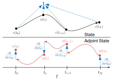
tldr: we can keep track of the $a$ variable which keeps track of $x(\tau )$ with AD, in the paper called reverse-mode differentiation

algorithm details

You solve a differential equation, that has the starting state of e.g. an image, and the end state - the function value at some point in time - is your classification. And at each point in time, the ODE solver queries the function for the gradient and solves it (???: minimizes it along some direction?)

$f_t$ is an equation defined by a neural network (green) and the (blue) arrows are the gradients at specific points in time.
$\theta \dots \text{parameters}$
But instead of going from input to output, this network parametrizes (learns) how you go from each step in time to the next (the gradient at each infinitesimally small timestep).

We start from the input layer $h(0)$ and we define the output layer $h(T)$ to be the solution to the ODE with initial value at some time $T$. An ODE solver calculates the necessary steps wherever necessary i.e. with arbitrary accuracy / time steps to achieve the desired accuracy (e.g. look at the ODE gradient field in the first figure: The black dots / points where the gradient was calculated are at arbitrary time intervals in contrast to the ResNet “which requires discretizing observation and emission intervals”).

The loss of the end state is equal to the loss of the start state plus the integral over time of the ODE $f$ given by and ODE solver:

$$\text{displaylines}L(z(t_1))=L\left(z(t_0)+{\int }_{t_0}^{t_1}f(z(t),t,\theta )dt\right)=L(\text{ODESolve}(z(t_0),f,t_0,t_1,\theta ))$$

The network doesn’t represent the continuous function, but is a discrete approximation to the linear update equation of ODEs (?)