Streaming Deep Reinforcement Learning Finally Works

year: 2024/10
paper: https://arxiv.org/pdf/2410.14606
website: https://x.com/RichardSSutton/status/1860818651953463542
code: https://github.com/mohmdelsayed/streaming-drl
connections: AMII, streaming RL, online learning

---

Extended Abstract (copypasta)

Although the prevalence of batch deep RL is often attributed to its sample efficiency, a more critical reason for the absence of streaming deep RL is its frequent instability and failure to learn, which we refer to as stream barrier. This paper introduces the stream-x algorithms, the first class of deep RL algorithms to overcome stream barrier for both prediction and control and match sample efficiency of batch RL

The agents, under the streaming reinforcement learning problem, are required to process one sample at a time without storing any samples for future reuse. Such requirements create additional hurdles compared to batch deep reinforcement learning, even though both learn from a non-stationary stream of data.
Streaming learning methods mainly require CPUs instead of GPUs since no batch updates are used, unless a very large neural network is used in which they might benefit from GPUs. In such case, the overhead of context switching between CPU and GPU might be negligible compared to the GPU computational cost required for the forward and backward passes in very large networks.

Issues that hinder learning:

1. learning instability due to occasional large updates,
2. learning instability due to activation nonstationarity, and
3. improper scaling of data

These issues are already present in batch methods causing several detrimental effects such as drop in performance, high variance, or inability to improve performance. However, they are exacerbated with streaming learning as updates can fluctuate more from one step to another due to non-i.i.d. sampling for updates. For example, streaming learning is more prone to instability as successive per-sample gradients can point in different directions, making it difficult to choose a single working step size. In contrast, batch methods mitigate this issue by averaging gradients from an i.i.d.-sampled batch drawn from a large pool.

3.1 Sample efficiency with sparse initialization and eligibility traces

Algorithm 1: SparseInit

$\text{Require: }\text{network }f\text{, sparsity level }s$

$$\begin{array}{rl}& \text{for weight }\mathbf{W}\text{ and bias }\mathbf{b}\text{ do}\\ & n\leftarrow s\times \text{fan\_in}\\ & \text{Permutation set }\mathcal{P}\text{ of size fan\_in}\\ & \text{Index set }\mathcal{I}\text{ of size }n\text{ (subset of }\mathcal{P}\text{)}\\ & W_{i,j}\sim U[-1/\sqrt{\text{fan\_in}},1/\sqrt{\text{fan\_in}}],\forall i,j\\ & W_{i,j}\leftarrow 0,\forall i\in \mathcal{I},\forall j\\ & b_i\leftarrow 0,\forall i\\ & \text{Return: }\text{initialized network }f\end{array}$$

In words: Initialize all weights and biases using LeCun Initialization, then set a random subset of those to 0.

3.2 Adjusting step sizes for maintaining update stability

In the streaming case, it is not clear if choosing a step size that reduces the error in the current sample is the best strategy. A more pertinent goal in streaming learning is to de-emphasize an update if it is too large, for example, if the update overshoots the target on a single sample.

Effective Step Size

Let $\delta (S)$ be the error on a sample before making an update (pre-update error). For TD-learning, this might be $r+\gamma v^{(s^{\prime })}-v^{(s)}$. Let ${\delta }^{+}(S)$ be the error on the same sample after making an update (post-update error).

The effective step size $\xi$ measures the relative amount of error correction:

$$\xi =\frac{\delta (S)-{\delta }^{+}(S)}{\delta (S)}$$

This quantity indicates how much of the original error was corrected by the update:
$\xi >1$ overshooting: The update was too aggressive, possibly changing the error’s sign
$\xi =1$ full correction: The update perfectly corrected the error
$\xi <1$ partial correction: The update made progress but did not overshoot
$\xi =0$ no correction: The update had no effect on the error
$\xi <0$ negative correction: The update made the error worse

E.g.:
$\delta =10,{\delta }^{+}=2\Rightarrow \xi =(10-2)/10=0.8$ (partial correction)
$\delta =10,{\delta }^{+}=-2\Rightarrow \xi =(10+2)/10=1.2$ (overshoot)

Algorithm 2: Bounding Effective Step Size with Backtracking (idealized optimizer)

$$\begin{array}{rlrl}& \text{Initialize: }\text{maximum effective step size }{\xi }_{\text{max}}\text{ (e.g., 0.05)}& & \\ & \text{Require: }\text{eligibility trace }{z}_w\text{, weight vector }w\text{, error function }\delta \text{, and starting step size }\alpha & & \\ & w^{\prime }\leftarrow w+\alpha {\delta }_w{z}_w& & ▹\text{ Counterfactual weights}\\ & \text{while }\frac{{\delta }_w-{\delta }_{w^{\prime }}}{{\delta }_w}>{\xi }_{\text{max}}\text{ do}& & ▹\text{ Exact effective step size detection}\\ & \alpha \leftarrow \beta \alpha & & ▹\text{ Backtracking line search until condition is met}\\ & w^{\prime }\leftarrow w+\alpha {\delta }_w{z}_w& & ▹\text{ Note that }{z}_w={\nabla }_{w}f\text{ for supervised learning}\\ & \text{return }{w}^{\prime }& & \end{array}$$

The algorithm prevents overshooting by adaptively reducing the step size until the effective step size is below a maximum threshold ${\xi }_{\text{max}}\in (0,1]$.
Small ${\xi }_{\max }\to 0$ conservative updates, ${\xi }_{\max }\to 1$ aggressive updates.

Backtracking line search is an optimization technique that starts with an initial step size $\alpha$ and progressively reduces it by a factor $\beta \in (0,1)$ until certain conditions are met. In this case, we keep reducing $\alpha$ until the effective step size $\xi$ falls below ${\xi }_{\text{max}}$. This is similar to classical line search methods, but here we’re focused on preventing overshooting on individual samples rather than optimizing a global objective.

For supervised learning, the eligibility trace ${\mathbf{z}}_w$ simplifies to ${\nabla }_{w}f$ because there’s no temporal component - we’re just trying to minimize error on individual input-output pairs. In reinforcement learning, eligibility traces serve a broader purpose by maintaining a decaying history of state visitations, helping to assign credit for rewards to earlier states.

The main drawback of this approach is that it requires multiple forward passes to compute ${\delta }^{+}$ for each new candidate step size. This can be expensive when many forward passes are required until we find a step size that satisfies the criteria.

Approximate Effective Step Size

To avoid the costly multiple forward passes required by the exact backtracking search, the authors use a first-order Taylor approximation, assuming local linearity (holds approximately when the updates are small, which is partly what we are aiming to achieve).
The post-update prediction for input $x$ can then be written as:

$$\begin{array}{rl}f(x;{\mathbf{w}}^{+})& =f(x;\mathbf{w}-\mathbf{u}(x;\mathbf{w}))\\ & =f(x;\mathbf{w})-{\nabla }_{\mathbf{w}}f(x;\mathbf{w}{)}^{\top }\mathbf{u}(x;\mathbf{w})\text{under local linearity}\end{array}$$

where ${\mathbf{w}}^{+}$ and $\mathbf{w}$ are parameters after and before the update, and $\mathbf{u}$ is the update vector.
For TD(λ), $\mathbf{u}=\alpha \delta \mathbf{z}$, where $\alpha$ is the step size, $\delta$ the TD error, and $\mathbf{z}$ the eligibility trace vector.
For supervised learning, $\mathbf{u}=\alpha {\nabla }_{\mathbf{w}}f$.

We use the already-computed gradients to compute the directional derivative, estimating changes due to a small weight update.

Local Linearity

f(x + \Delta x) \approx f(x) + f’(x)\Delta x

$$Thisapproximationbecomeslessaccurateasupdatesgetlarger,whichiswhywewanttokeepupdatessmallinthefirstplace.Forneuralnetworks,thismeanswecanapproximatehowthepredictionwillchangeafteraweightupdatewithoutactuallyhavingtorunanotherforwardpassthroughthenetwork.$$

This leaves us with the following effective step size for TD($\lambda$) under nonlinear function approximation:

$$\begin{array}{rl}\xi & =\frac{(r+\gamma v(\mathbf{w};{\mathbf{x}}^{\prime })-v(\mathbf{w};\mathbf{x}))-(r+\gamma v({\mathbf{w}}_{+};{\mathbf{x}}^{\prime })-v({\mathbf{w}}_{+};\mathbf{x}))}{\delta }\\ & =\frac{\alpha \delta \gamma {\mathbf{z}}^T{\nabla }_{\mathbf{w}}v(\mathbf{w};{\mathbf{x}}^{\prime })-\alpha \delta {\mathbf{z}}^T{\nabla }_{\mathbf{w}}v(\mathbf{w};\mathbf{x})}{\delta }\\ & =\alpha {\mathbf{z}}^T(\gamma {\nabla }_{\mathbf{w}}v(\mathbf{w};{\mathbf{x}}^{\prime })-{\nabla }_{\mathbf{w}}v(\mathbf{w};\mathbf{x}))\end{array}$$

We compute the TD-error on a sample before and after the update, and divide the difference by the original error to get the effective step size.
This would still require an additional backward pass for the value function at the next state ${\mathbf{x}}^{\prime }$, so we further approximate the effective step size:

$$\begin{array}{rl}\xi & =\alpha {\mathbf{z}}^T(\gamma {\nabla }_{\mathbf{w}}v(\mathbf{w};{\mathbf{x}}^{\prime })-{\nabla }_{\mathbf{w}}v(\mathbf{w};\mathbf{x}))\\ & \le \alpha |\mathbf{z}{|}^T{\nabla }_{\mathbf{w}}|\gamma v(\mathbf{w};{\mathbf{x}}^{\prime })-{\nabla }_{\mathbf{w}}v(\mathbf{w};\mathbf{x})|\le \alpha |\mathbf{z}{|}^{T}1\\ & =\alpha \Vert \mathbf{z}{\Vert }_1\le \kappa \alpha \Vert \mathbf{z}{\Vert }_1,\text{where }\kappa >1\\ & \le \kappa \alpha \bar{\delta }\Vert \mathbf{z}{\Vert }_1,\text{where }\bar{\delta }=\max (|\delta |,1)\end{array}$$

[!note] Approximate Effective Step Size

To avoid multiple forward passes in the exact backtracking method, the paper uses a first-order Taylor approximation under a local linearity assumption. For small updates, we can estimate how much the network output changes using only the gradient at the current weights. This is cheaper than performing another forward or backward pass.

When we update weights from $\mathbf{w}$ to ${\mathbf{w}}^{+}$ by a vector $\mathbf{u}$, local linearity tells us

$$\begin{array}{rl}f(x;{\mathbf{w}}^{+})& =f(\mathbf{x};\mathbf{w}-\mathbf{u}(\mathbf{x};\mathbf{w}))\\ & \approx f(x;\mathbf{w})-{\nabla }_{\mathbf{w}}f(x;\mathbf{w}{)}^{\top }\mathbf{u}(x;\mathbf{w})\text{under local linearity}\end{array}$$

For TD(λ), $\mathbf{u}=\alpha \delta \mathbf{z}$, where $\alpha$ is the step size, $\delta$ the TD error, and $\mathbf{z}$ the eligibility trace vector.
For supervised learning, $\mathbf{u}=\alpha {\nabla }_{\mathbf{w}}f$.
This approximation avoids re-running a full forward pass at the new weights, because the directional derivative in the above equation only needs the existing gradient. The local linearity assumption holds / the approximation is most accurate when the update $\mathbf{u}$ is small, which aligns with our goal of preventing large, destabilizing steps.

Local Linearity f as if it is linear in a small neighborhood around w. Formally, for small ∆w:

f(x; \boldsymbol{w} + \Delta \boldsymbol{w}) \approx f(x; \boldsymbol{w}) + \nabla_{\boldsymbol{w}} f(x; \boldsymbol{w})^\top \Delta \boldsymbol{w}

$$Thisworksbestwhen\Vert ∆w\Vert issmall.Itisthesameideaasapproximatingacurvebyitstangentlineatapoint.$$

In TD-learning, the error $\delta$ depends on both the current state $x$ and the next state $x\prime$:

$$\delta =r+\gamma v(\mathbf{w};x^{\prime })-v(\mathbf{w};x)$$

After the update, the new error ${\delta }^{+}$ depends on $w^{+}$. The effective step size $\xi$ is defined as

$$\xi =\frac{\delta -{\delta }^{+}}{\delta }$$

Computing ${\delta }^{+}$ exactly at $x\prime$ and $w^{+}$ would require an extra backward pass. Instead, the paper uses local linearity to approximate how $v$ changes at $x$ and $x^{\prime }$, yielding

$$\begin{array}{rl}\xi & =\frac{(r+\gamma v(\mathbf{w};{\mathbf{x}}^{\prime })-v(\mathbf{w};\mathbf{x}))-(r+\gamma v({\mathbf{w}}_{+};{\mathbf{x}}^{\prime })-v({\mathbf{w}}_{+};\mathbf{x}))}{\delta }\\ & =\frac{\alpha \delta \gamma {\mathbf{z}}^T{\nabla }_{\mathbf{w}}v(\mathbf{w};{\mathbf{x}}^{\prime })-\alpha \delta {\mathbf{z}}^T{\nabla }_{\mathbf{w}}v(\mathbf{w};\mathbf{x})}{\delta }\\ & =\alpha {\mathbf{z}}^{\top }(\gamma {\nabla }_{\mathbf{w}}v(\mathbf{w};x^{\prime })-{\nabla }_{\mathbf{w}}v(\mathbf{w};x))\end{array}$$

Even this approximation requires computing a new gradient at $x^{\prime }$. We can avoid this by deriving a bound: The difference between gradients at nearby states can’t be too large (Lipschitz continuity), and for nearby states with discount factor close to 1, this difference is at most 1.
This lets us bound the effective step size using just the L1 norm of the eligibility trace: $\xi \le \kappa \alpha \bar{\delta }\Vert \mathbf{z}{\Vert }_1$

This bound tells us that to prevent overshooting, we should scale down our step size when the eligibility traces have large magnitude $\Vert \mathbf{z}{\Vert }_1$ or $\bar{\delta }$ is large.

$$\begin{array}{rl}\xi & =\alpha {\mathbf{z}}^T(\gamma {\nabla }_{\mathbf{w}}v(\mathbf{w};{\mathbf{x}}^{\prime })-{\nabla }_{\mathbf{w}}v(\mathbf{w};\mathbf{x}))\\ & \le \alpha |\mathbf{z}{|}^T{\nabla }_{\mathbf{w}}|\gamma v(\mathbf{w};{\mathbf{x}}^{\prime })-{\nabla }_{\mathbf{w}}v(\mathbf{w};\mathbf{x})|\le \alpha |\mathbf{z}{|}^{T}1\\ & =\alpha \Vert \mathbf{z}{\Vert }_1\le \kappa \alpha \Vert \mathbf{z}{\Vert }_1,\text{where }\kappa >1\\ & \le \kappa \alpha \bar{\delta }\Vert \mathbf{z}{\Vert }_1,\text{where }\bar{\delta }=\max (|\delta |,1)\end{array}$$

Extra notes on bounding $\left|\gamma \right[{\nabla }_{\mathbf{w}}v(\mathbf{w};x^{\prime }){]}_i-[{\nabla }_{\mathbf{w}}v(\mathbf{w};x){]}_i|\le 1$ Note: $|\mathbf{z}{|}^{\top }1=\Vert \mathbf{z}{\Vert }_1$ They do this because something something lipschitz continuity of gradients tells us that nearby states will have similar gradients something something. $\bar{\delta }$ exists so that if $\delta$ is very small, the bound does not become trivial. $\kappa$ exists so … ???

Algorithm 3: Overshooting-bounded Gradient Descent (ObGD)

$$\begin{array}{rl}\text{Require: }& \text{eligibility trace }{\mathbf{z}}_w\text{, weight vector }\mathbf{w}\text{, error }\delta \text{, step size }\alpha \text{, scaling factor }\kappa \\ \bar{\delta }& \leftarrow \max (|\delta |,1)\\ M& \leftarrow \kappa \alpha \bar{\delta }\Vert {\mathbf{z}}_w{\Vert }_1▹\text{ Note that }{\mathbf{z}}_w={\nabla }_{w}f\text{ for supervised learning}\\ \alpha & \leftarrow \min (\frac{\alpha }{M},\alpha )\\ \mathbf{w}& \leftarrow \mathbf{w}+\alpha \delta {\mathbf{z}}_w\\ \text{return }\mathbf{w}& \end{array}$$

This algorithm avoids the need for multiple forward passes by directly scaling the step size based on the theoretical bound of the effective step size. The scaling ensures updates remain controlled without requiring backtracking.

The key idea is to scale down the step size $\alpha$ based on:

• How large the current error $\delta$ is, $\bar{\delta }$)
• How “steep” the current update direction is ($\Vert {\mathbf{z}}_w{\Vert }_1$)
• A safety factor $\kappa$ that accounts for potential nonlinearity

3.3 Stabilizing activation distribution under non-stationarity

→ They use layer normalization (applied to the pre-activation of each layer (before applying the activation $\sigma$))

3.4 Proper scaling of data

They use Welfords method to scale observations and rewards.

Algorithm 4: SampleMeanVar

Transclude of Welfords-method#^5e7046

Algorithm 5: Scale Reward

$$\begin{array}{rl}\text{Initialize: }& u\leftarrow 0\\ \text{Require: }& r,\gamma ,p,T,n\\ u& \leftarrow \gamma (1-T)u+r\\ \_,p,{\sigma }^2,n& \leftarrow \text{SampleMeanVar}(u,0,p,n)\\ \text{Return: }& \frac{u-p}{\sqrt{{\sigma }^2+ϵ}},p\end{array}$$

Algorithm 6: NormalizeObservation

$$\begin{array}{rl}\text{Require: }& S,\mu ,p,n\\ \mu ,{\sigma }^2,p,n,& \leftarrow \text{SampleMeanVar}(S,\mu ,p,n)\\ \text{Return: }& \frac{S-\mu }{\sqrt{{\sigma }^2+ϵ}},\mu ,p,n\end{array}$$

3.5 Stable streaming deep reinforcement learning methods

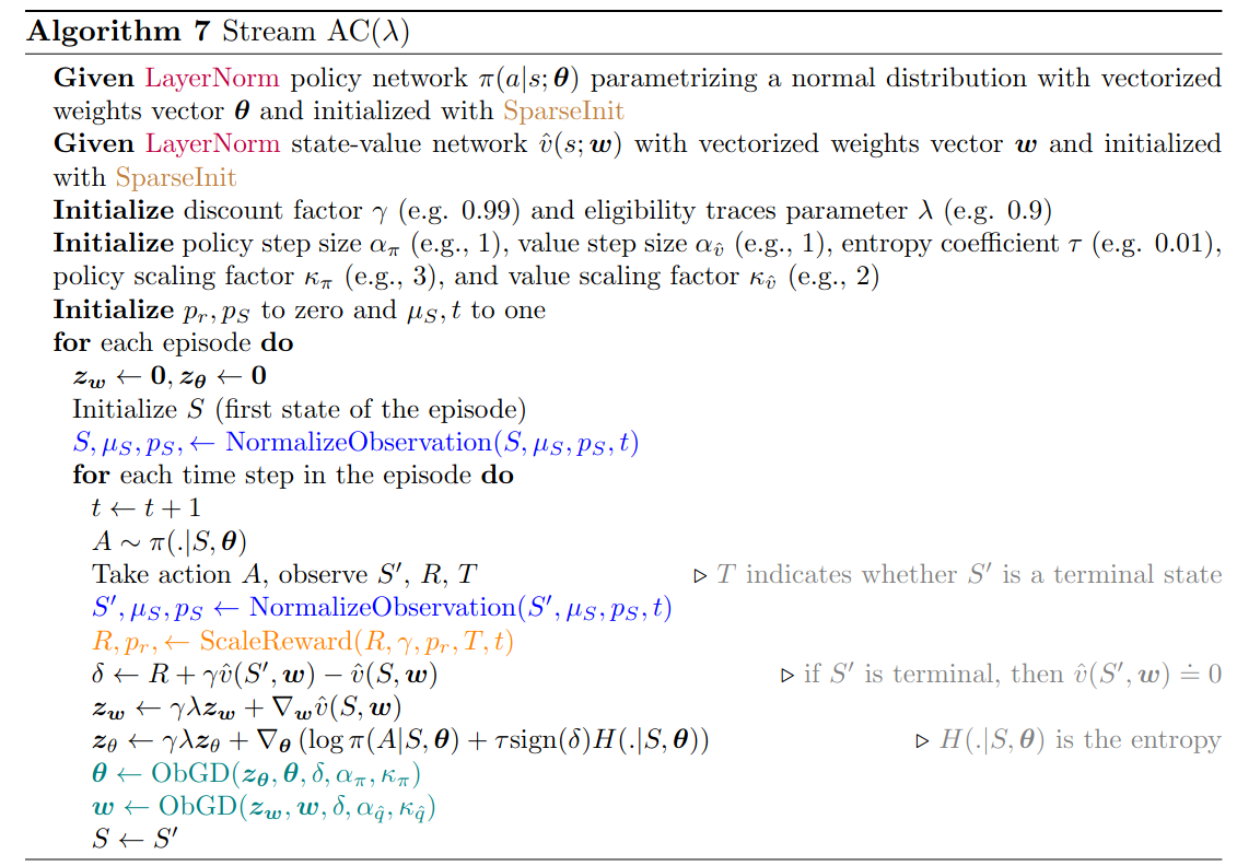
$\theta$ is the actor, $w$ is the critic