TD Lambda

The question of what $n$ we want to pick, i.e. how soon to start relying on predicted rewards, is handled by TD Lambda in a similar way / with a similar intuition as with reward discounting: We take a weighted average of all possible $n$-step TD targets rather than picking a single best $n$, discounting future rewards, as the further in the future we predict, the less confident we are.

Link to original

TD$(\lambda )$ decays the n-step return by a factor $0\le \lambda <1$:

$$G_t^{\lambda }=(1-\lambda )\sum _{n=1}^{\infty }{\lambda }^{n-1}{G}_t^{(n)}$$

We multiply by $(1-\lambda )$ to normalize the lambdas, i.e form a weighted average, which follows from rearranging the geometric sequence:

$$\begin{array}{rl}\Lambda & =1+\lambda +{\lambda }^2+\dots \\ \Lambda & =1+\lambda (1+\lambda +{\lambda }^2)\\ \Lambda & =1+\lambda \Lambda \\ \Lambda -\lambda \Lambda & =1\\ (1-\lambda )\cdot \Lambda & =1\end{array}$$

This is different to $\gamma$ discounting, where we want future rewards to have less total influence and thus don’t normalize the weights – the infinite sum ${\sum }_{k=0}^{\infty }{\gamma }^k=\frac{1}{1-\gamma }$ represents the maximum possible return rather than forming a weighted average of complete estimates.

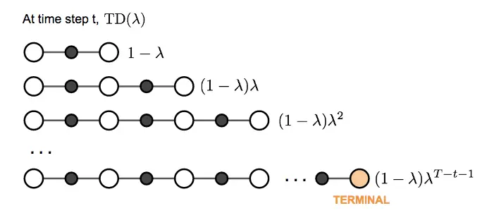
TD(0) is equivalent to using only a single step actual reward and predicting the next.
TD($\infty$) is equivalent to monte carlo methods (complete trajectories of actual rewards).

TD lambda smoothly interpolates between on- and off-policy: Large $\lambda$ → close to on-policy, small $\lambda$ → close to off-policy.

The higher $\lambda$, the less bias, but the more variance, and vice versa.

Implementation:

def get_tdlambda_returns_and_advantages(
		rewards: Float[np.ndarray, "steps ..."],
		values: Float[np.ndarray, "step ..."],
		dones: Float[np.ndarray, "steps ..."],
		gamma: float,
		lambda_param: float,
) -> tuple[Float[np.ndarray, "steps ..."], Float[np.ndarray, "steps ..."]]:
	"""Compute returns and advantages using TD(λ)"""
	steps = rewards.shape[0]
	returns = np.zeros_like(rewards)
	nonterminal_mask = 1 - dones
	
	# Initialize last return for bootstrapping
	last_return = values[-1]
	
	# Compute λ-returns going backwards
	for t in reversed(range(steps)):
		# TD target = r_t + γV(s_{t+1})
		td_target = rewards[t] + gamma * values[t + 1] * nonterminal_mask[t]
		# Blend immediate TD target with bootstrapped future return
		returns[t] = td_target * (1 - lambda_param) + (gamma * lambda_param * last_return * nonterminal_mask[t])
		last_return = returns[t]
	
	advantages = returns - values[:-1]
	return returns, advantages

Eligibility traces provide an online, incremental way to implement TD(λ)

There are two equivalent ways to understand TD(λ):
The “forward view” (TD(λ) original formulation):

$$G_t^{\lambda }=(1-\lambda )\sum _{n=1}^{\infty }{\lambda }^{n-1}{G}_t^{(n)}$$

This looks ahead at future rewards, combining n-step returns with weights that decay by λ. While theoretically elegant, it’s not practical for online learning since you need to wait for future rewards.
The “backward view” (eligibility traces):

$$\begin{array}{rl}{w}_{t+1}& =w_t+\alpha {\delta }_t{z}_t\\ z_t& =\gamma \lambda z_{t-1}+{\nabla }_w\hat{v}(S_t,w_t)\end{array}$$

This maintains a trace of past gradients, allowing immediate updates. It’s more practical for implementation.
Think of it like integration vs. summation:
The forward view (TD(λ)) is like calculating an area under a curve by looking at the whole curve.
The backward view (eligibility traces) is like approximating the same area by accumulating small rectangular slices as you go.
→ Rather than having to wait for future rewards to compute the λ-return, the trace maintains an exponentially-weighted sum of past gradients that approximates the same multi-step update. This makes them particularly valuable for continuous learning scenarios where we want to learn from partial trajectories.

---

The one-step TD error ${\delta }_t$ for value estimates is defined as:

$${\delta }_t=R_{t+1}+\gamma \hat{v}(S_{t+1},w)-\hat{v}(S_t,w)$$

Each n-step return can be decomposed into a sum of TD errors:

$$G_t^{(n)}-\hat{v}(S_t,w)=\sum _{k=t}^{t+n-1}{\gamma }^{k-t}{\delta }_k$$

Substituting this into the forward view equation and rearranging:

$$G_t^{\lambda }-\hat{v}(S_t,w)=\sum _{k=t}^{\infty }(\gamma \lambda {)}^{k-t}{\delta }_k$$

For linear function approximation where $\hat{v}(s,w)=w^T\varphi (s)$, $\varphi (s)$ … feature vector representing state $s$, the forward view update:

$$w_{t+1}=w_t+\alpha (G_t^{\lambda }-\hat{v}(S_t,w)){\nabla }_w\hat{v}(S_t,w)$$

becomes equivalent to the backward view with eligibility traces:

$$\begin{array}{rl}{w}_{t+1}& =w_t+\alpha {\delta }_t{z}_t\\ z_t& =\gamma \lambda z_{t-1}+{\nabla }_w\hat{v}(S_t,w)\end{array}$$

The trace $z_t$ recursively accumulates exactly the information needed to implement the forward view, but does so incrementally without having to wait for future rewards. This equivalence holds exactly for linear function approximation, which partly explains why eligibility traces have been most successful in linear or tabular settings.

Link to original