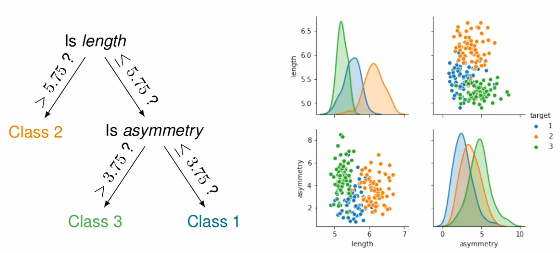
Decision Tree
A decision tree is a supervised learning algorithm that classifies (or regresses) by recursively partitioning the feature space with axis-aligned splits. Each internal node tests a feature against a threshold, each branch represents the outcome, and each leaf holds a prediction.
Given data , the tree is built top-down by greedily choosing the split (feature , threshold ) that best separates classes.
For classification, leaves predict the majority class among samples that reach them; for regression, the mean target value.
The tree structure makes predictions interpretable—you can trace exactly which feature comparisons led to a decision, and features used early/often indicate importance.

Construction (greedy recursive partitioning)
Start with all training samples at the root node
Find the best split: try all features and thresholds, pick the one that maximizes purity gain (see splitting criteria below)
Partition samples into child nodes based on the split
Recurse on each child until a stopping criterion is met (max depth, min samples, pure node, etc.)
This greedy approach doesn’t guarantee the globally optimal tree—an early split that looks good might prevent better splits downstream. But exhaustive search over all possible trees is computationally intractable.
Splitting criteria
At each node, we want splits that make child nodes “purer” (more homogeneous in class). Common measures:
Gini impurity: — the probability of misclassifying a randomly chosen element if labeled according to the class distribution. A pure node (single class) has .
Entropy / information gain (ID3, C4.5): . The split maximizing is chosen.
Both are concave functions that peak at uniform distributions and hit zero for pure nodes. Gini is slightly faster to compute; entropy penalizes impure nodes a bit more strongly.
Overfitting and regularization
A fully grown tree can perfectly classify training data by creating one leaf per sample, i.e. extreme overfitting.
Single decision trees have notoriously high variance: small changes in training data can produce completely different tree structures.Pre-pruning (stopping criteria): Limit growth via max depth, minimum samples per leaf/split, or minimum impurity decrease.
Post-pruning: Grow the full tree, then collapse subtrees that don’t improve validation performance. More expensive but often more effective.
But more commonly, ensembles of trees (like random forests or gradient boosting machines) are used to reduce variance and improve generalization; the averaging over many overfit trees dramatically reduces variance while preserving the low bias of deep trees.
Properties
Interpretable: You can inspect exactly how predictions are made—trace the path from root to leaf. Feature importance is visible from which features appear in splits (and how early).
No distance metric needed: Unlike k-NN or k-means, decision trees use only feature comparisons, making them invariant to feature scaling and able to naturally mix continuous and categorical features.
Missing values: Can be handled via surrogate splits (finding alternative features that approximate the original split).
Limitations
Axis-aligned boundaries: Each split asks “is feature ?” — geometrically, this cuts the feature space with a line perpendicular to that feature’s axis. If the true decision boundary is diagonal (e.g., “class A when ”), the tree must approximate it with a staircase of many horizontal and vertical cuts. This leads to unnecessarily deep trees and poor generalization on such problems. Methods like SVMs can directly learn diagonal (or curved) boundaries.
Instability: The greedy, hierarchical construction means early splits constrain all subsequent ones. A slightly different dataset can produce a completely different root split, cascading into an entirely different tree structure—hence the high variance.