year: 2017
paper: https://sebastianrisi.com/wp-content/uploads/nichele_tcds2017.pdf
website:
code:
connections: CA, NEAT, CPPN, self-organization, morphogenesis, developmental encoding, Sebastian Risi, Stefano Nichele
In a nutshell
- CA-NEAT evolves CPPNs (as the CA’s transition rule) with NEAT, so a single genome maps local neighborhood states → next state. Phenotypes then emerge via self-organization. Targets: 2D morphogenesis and replication benchmarks.
- CPPNs scale linearly with neighborhood size and # states unlike exponential CA rule tables, and NEAT lets genomes complexify only as needed.
- i.e. if you add a state, you only need to add one output node to the CPPN, if you add a neighbor, you only need to add one more input node.
- morphogenesis: on a fixed toroidal grid, i.e. no borders
- evaluate best match within 30 steps.
- downweights trivial all-empty attractors
- replication: on an auto-expanding grid, so copies aren’t cut at edges
- score top-3 non-overlapping matches per step;
- imperfect replicas discounted
- von Neumann neighborhood
- 100 runs per task
- pop. 200
- speciation & sigma-scaled selection
Main takeaways from experiments:
- Simple patterns (Mosaic): solved in gen 0-1 — the target has strong local regularity (repeating tiles), so even minimal CPPNs with no hidden nodes can encode it
- Deceptive patterns (Border): only ~1% success by gen 500 — evolution finds “almost correct” frames (one cell off) that score well but can’t escape these local optima to reach the perfect frame
- Pattern difficulty varies by task type: Swiss is easier for replication than morphogenesis; Tricolor shows opposite trend
- Long-range coordination is the bottleneck: Nordic replication fails completely — the pattern requires precise timing/phase across distant cells, which von Neumann neighborhood + local rules struggle to coordinate. Mosaic/Swiss succeed because they’re compositional from local building blocks
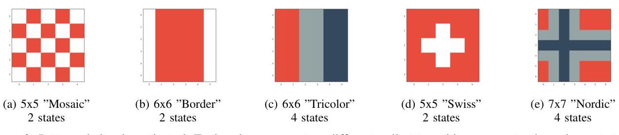
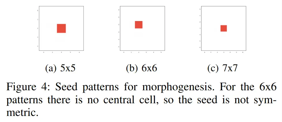
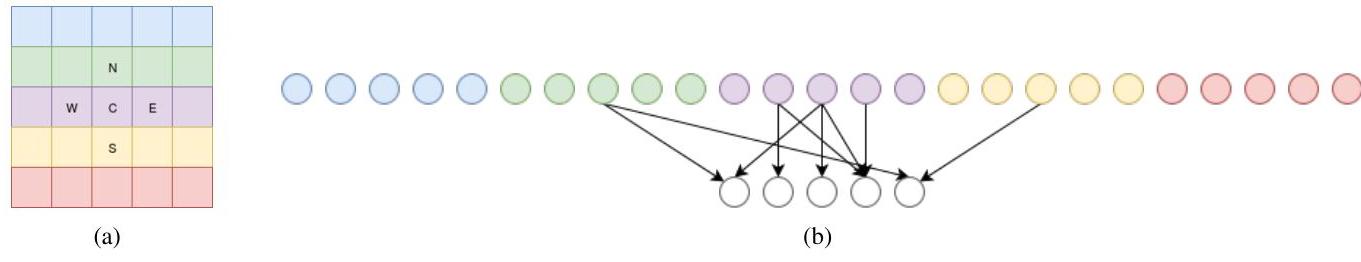
Figure 17: An example CPPN with a large available input neighbourhood, but only the Von Neumann sub-neighbourhood connected to the output layer.
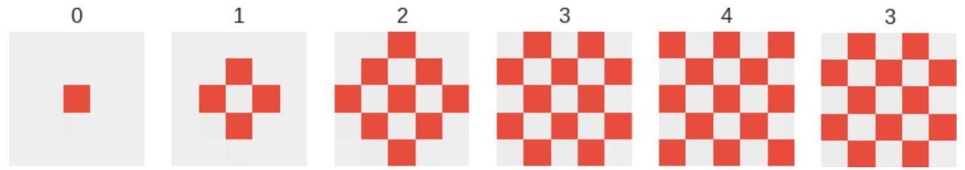
Figure A.1: A solution to the ”Mosaic” morphogenesis where the CA finds a two-step cycle that includes the target pattern
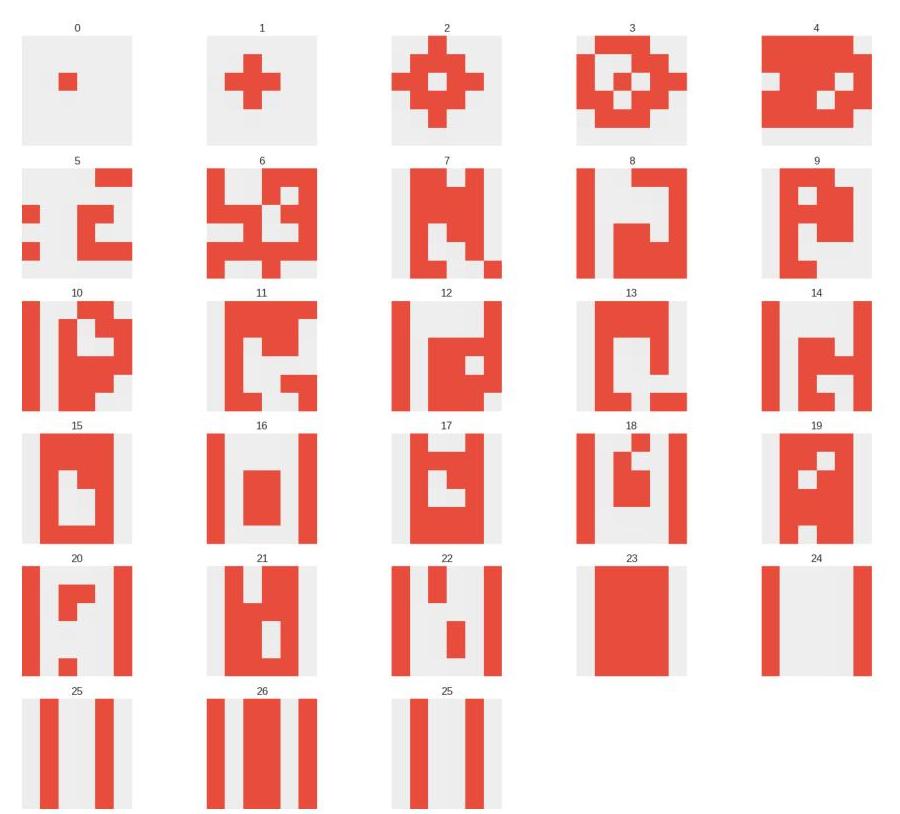
Figure A.5: The only solution that was found for the ”Border” morphogenesis. After finding the target state in iteration 23, the CA goes in to a two-step cycle which does not include the target state.
Extra details
When the initial population is created, the number of connections for each individual is randomly initialised to be between 50% and 100% of being fully connected.
During development of the system, a variation of different configurations was tested for different problems. However, for the results included herein, a choice was made to use the same CPPN-NEAT configuration, and as close to the same CA configuration as possible for all problems. This makes it easier to make comparison between experiments, but also means that the settings chosen may favour some experiments over others. The optimisation of CPPN-NEAT parameters is outside the scope of this paper.