marginalization

Marginal density

The marginal density of a variable is obtained by integrating the joint density over the other variable:

$$\begin{array}{rl}{f}_X(x)& ={\int }_{-\infty }^{\infty }f(x,y)dy\end{array}$$

Here we’re integrating out (averaging over all possible values of) $Y$, to get the marginal density of $X$, i.e. the density of $X$ regardless of $Y$.
This also work with discrete distributions: $P(X=x)={\sum }_{i}P(X=x,Y=y_i)$

Link to original

Marginalization and conditioning

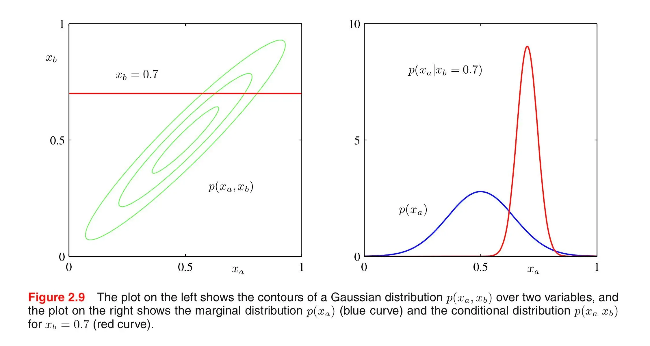
Gaussian distributions are closed under marginalization and conditioning, i.e. they return a modified gaussian distribution.
E.g. for the following bivariate distribution:

$$P_{X,Y}=\left[\begin{array}{c}X\\ Y\end{array}\right]\sim N(\mu ,\Sigma )=\mathcal{N}(\left[\begin{array}{c}{\mu }_X\\ {\mu }_Y\end{array}\right],\left[\begin{array}{cc}{\Sigma }_{XX}& {\Sigma }_{XY}\\ {\Sigma }_{YX}& {\Sigma }_{YY}\end{array}\right])$$

Marginalization

Marginalization lets us extract partial information from multivariate probability distributions. Given a normal probability distribution $P(X,Y)$ over vectors of random variables $X$ and $Y$, we can determine their marginalized probability distributions like this:

$$\begin{array}{rl}X& \sim \mathcal{N}({\mu }_X,\Sigma XX)\\ Y& \sim \mathcal{N}({\mu }_Y,{\Sigma }_{YY})\end{array}$$

This means that each partition $X$ and $Y$ only depends on its corresponding entries in $\mu$ and $\Sigma$.

Another way to express this, mathematically, is that we view every possible value of $X$ under the consideration of all possible values of $Y$, e.g.: $P(X=x_1)=P(X=x_1,Y=y_1)+\cdots +P(X=x_1,Y=y_n))$, everaging out Y’s contribution:

$$p_X(x)={\int }_y{p}_{X,Y}(x,y)dy={\int }_y{p}_{X|Y}(x|y)p_Y(y)dy$$

Conditioning

Conditioning is used to determine the probability distribution of one variable depending on another variable, i.e. how one variable behaves when another one is known.

$$\begin{array}{rl}X|Y& \sim \mathcal{N}({\mu }_X+{\Sigma }_{XY}{\Sigma }_{YY}^{-1}(Y-{\mu }_Y),{\Sigma }_{XX}-{\Sigma }_{XY}{\Sigma }_{YY}^{-1}{\Sigma }_{YX})\\ Y|X& \sim \mathcal{N}({\mu }_Y+{\Sigma }_{YX}{\Sigma }_{XX}^{-1}(X-{\mu }_X),{\Sigma }_{YY}-{\Sigma }_{YX}{\Sigma }_{XX}^{-1}{\Sigma }_{XY})\end{array}$$

The mean gets shifted by how much the known variable differs from its expected value $(Y-{\mu }_Y)$ , which is normalized by ${\Sigma }_{YY}^{-1}$ (think $(Y-{\mu }_y)/Y$), and scaled by the covariance between the two variables ${\Sigma }_{XY}$ . This product can be thought of as translating the normalized deviation in $Y$ to corresponding changes in $X$’s scale.
→ ${\Sigma }_{XY}{\Sigma }_{YY}^{-1}{\Sigma }_{YX}$ represents the amount of variance in $X$ that can be explained by $Y$.

Conditioning is like taking a slice of the distribution at the known/given value of a variable.

Visualization of marginalization and conditioning

Note: There is an interactive version at distill.

The blue curve shows the entire underlying distribution of the random variable $x_a$, and the red curve shows a slice of the joint distribution of $x_a$ and $x_b$ at a specific value of $x_b$.
i

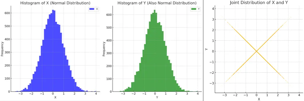
For normal distributions, uncorrelated variables are independent if and only if they are jointly normally distributed.

A pair $(X,Y)$ is jointly normal exactly when every linear combination $aX+bY$ is normally distributed, i.e. the resulting distribution is a multivariate normal distribution.

Visual intuition $X\sim \mathcal{N}(0,1)$ and $Y=WX$ where $W$ is $\pm 1$ with equal probability:

Consider

Individually $X$ and $Y$ each look normal, but together their joint distribution is unusual: When $X$ is positive, $Y$ is either $+X$ or $-X$ with 50/50 chance, when $X$ is negative, same thing.

→ $X$ and $Y$ cannot possibly be independent, even though they’re uncorrelated!

Link to original