General intelligence requires rethinking exploration

year: 2023/06
paper: https://royalsocietypublishing.org/doi/full/10.1098/rsos.230539
website:
code:
connections: generalization, intelligence, general intelligence, open-ended, exploration, RL, SL, novelty, exploration vs exploitation

---

Takeaways

• Open-ended exploration == exploring the space of MDPs.
• Separating exploitation (task) from exploration (data collection) is very useful (bootstrap problem, …).
• SL can be open-ended, if we involve an active data collection process.
• Offline vs online collection is secondary, key is to actively collect, i.e. to gather diverse, grounded data with high learning potential.

A relative notion of general intelligence | Increasingly general intelligence (IGI)

Model A is more general than model B relative to a task set T if and only if A performs above a threshold level (e.g. that of a minimally viable solution) in more tasks in T than B, while at least matching the performance of B on all other tasks in T on which B meets the threshold.
Under this definition, general intelligence is not necessarily the end state of any system, but rather a property that can change over time, relative to other intelligent systems and the specific task domain. We can then refer to a system exhibiting continual improvements in relative general intelligence as an increasingly general intelligence (IGI).
… we do not aim to address whether the notion of a general intelligence relative to the space of all possible tasks is well defined, as it is an orthogonal concern to the argument we lay out in this paper.

Open-ended exploration

The problem afflicting both classes of learning algorithms reduces to one of insufficient exploration: SL, largely trapped in the offline regime, fails to perform any exploration, while RL, limited to exploring the interior of a static simulation, largely ignores the greater expanse of possibilities that the simulation cannot express.
We require a more general kind of exploration, which searches beyond the confines of a static data generator, such as a finite dataset or static simulator. This generalized form of exploration must deliberately and continually seek out promising data to expand the learning agent’s repertoire of capabilities. Such expansion necessarily entails searching outside of what can be sampled from a static data generator.
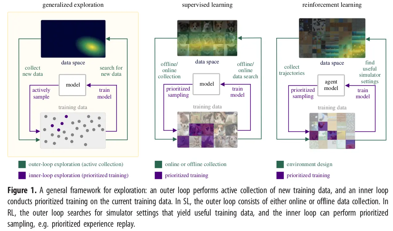
This open-ended exploration process, summarized in figure 1, defines a new data-seeking outer-loop that continually expands the data generator used by the inner loop learning process, which itself may use more limited forms of exploration to optimally sample from this data generator. Within each inner loop, the data generator is static, but as a whole, this open-ended exploration process defines a dynamic, adaptive search process that generates the data necessary for training a likewise open-ended learner that, over time, may attain increasingly general capabilities.

Supervised Learning (SL)

Supervised learning aims to learn a function $f$ mapping points in domain $\mathcal{X}$ to domain $\mathcal{Y}$ given $N$ training examples $(x_i,y_i{)}_{i=0}^N$ reflecting this mapping, where $x_i\in \mathcal{X}$ and $y_i\in \mathcal{Y}$.
In modern ML, this function is typically a large ANN with parameters denoted $\theta \in \Theta$.
The defining feature of SL is that learning proceeds by optimizing a loss function $\mathcal{L}:\Theta \times \mathcal{X}\times \mathcal{Y}\to \mathbb{R}$ that provides the error between the model’s prediction $f(x)$ and the true value $y$ paired with $x$. In general, each training example $(x,y)$ can be seen as a sample from a ground-truth distribution $P(x,y)$, because the true data generating function $f^{\ast }:\mathcal{X}\to \mathcal{Y}$ can be stochastic. Therefore, the goal of SL can be seen as learning an approximator $f:\mathcal{X}\to \mathcal{Y}$ that produces samples $y$ consistent with $P(y|x)$, for example, by using a loss function that encourages $f$ to deterministically predict the mean or mode of $P(y|x)$, or that matches the distribution of outputs of $f(x)$ to $P(y|x)$.

Crucially, this definition of SL assumes the model $f$ is trained once on a static, finite training dataset ${\mathcal{D}}_{\text{train}}$. We should thus not expect $f$ to accurately model data that differs significantly from its training data.

---

Nevertheless, with massive amounts of training data, large models can exhibit impressive generality and recent scaling laws suggest that test performance should improve further with even more data. Given the benefits of data scale, contemporary state-of-the-art SL models are trained on internet-scale, offline datasets, typically harvested via webcrawling.

While such datasets may capture an impressive amount of information about the world, they inevitably fall short in containing all relevant information that a model may need when deployed in the wild. All finite, offline datasets share two key shortcomings: incompleteness, as the set of all facts about the world is infinite, and stationarity, as such datasets are by definition fixed.
For example, our virtual assistant, if trained on a static conversational corpus, would soon see its predictions grow irrelevant, as its model falls out of date with culture, world events, and even language usage itself. Indeed, all ML systems deployed in an open-world setting, with real users and peers, must continually explore and train on new data, or risk fading into irrelevance. What data should the system designer (or the system itself ) collect next for further training? This is the complementary — and equally important — problem of exploration that sits beneath all ML systems in deployment, one that has been considered at length in the field of RL. ¹

Link to original

Limitations of RL

As RL agents train on their own experiences, locally optimal behaviours can easily self-reinforce, preventing the agent from reaching better optima. To avoid such outcomes and ensure sufficient coverage of possible MDP transitions during training, RL considers exploration a principal aim.

Under exploration, the RL agent performs actions in order to maximize some measure of novelty of the resulting experiential data or uncertainty in outcome, rather than to maximize return (ICM, CEED. Simpler still, new and informative states can often be unlocked by injecting noise into the policy, e.g. by sporadically sampling actions uniformly at random (see epsilon greedy, PPO). However, such random search strategies (also ES) can run into the curse of dimensionality, becoming less sample efficient in practice.

A prominent limitation of state-of-the-art RL methods is their need for large amounts of data to learn optimal policies. This sample inefficiency is often attributable to the sparse-reward nature of many RL environments, where the agent only receives a reward signal upon performing some desired behaviour. Even in a dense reward setting, the agent may likewise see sample-inefficient learning once trapped in a local optimum, as discovering pockets of higher reward can be akin to finding a similarly sparse signal.

In complex real-world domains with large state spaces and highly branching trajectories, finding the optimal behaviour may require an astronomical number of environment interactions, despite performing exploration. Thus for many tasks, training an RL agent using real-world interactions is highly costly, if not completely infeasible. Moreover, a poorly trained embodied agent acting in real-world environments can potentially perform unsafe interactions. For these reasons, RL is typically performed within a simulator, with which massive parallelization can achieve billions of samples within a few hours of training.
Simulation frees RL from the constraints of real-world training at the cost of the sim2real gap, the difference between the experiences available in the simulator and those in reality. When the sim2real gap is high, RL agents perform poorly in the real world, despite succeeding in simulation. Importantly, a simulator that only implements a single task or small variations thereof will not produce agents that transfer to the countless tasks of interest for general intelligence. Thus, RL ultimately runs into a similar data limitation as in SL.
In fact, the situation may be orders of magnitude worse for RL, where unlike in SL, we have not witnessed results supporting a power-law scaling of test loss on new tasks, as a function of the amount of training data. Existing static RL simulators may thus impose a more severe data limitation than static datasets, which have been shown capable of inducing strong generalization performance. ¹

Link to original

Generalized/Open-ended exploration and learning.

Generalized exploration is a data collection process that seeks to explore the full space of possible input data to the model.
When this data space is unbounded, we may say the process performs open-ended exploration.
A nodel trained on such a data stream then performs open-ended learning.

Though RL considers the problem of exploration, existing methods insufficiently address this form of data collection

The simulator ( MDP) in RL plays an analogous role to the training data in RL

Both define some distribution $\mathcal{D}$ over the space of available training data.

SL: $\mathcal{D}\sim \mathcal{U}\{(x_i,y_i)\}$ … uniform distribution over datapoints, where $(x_i,y_i)\sim P(X,Y)$.

RL: Simulator returns a training trajectory $\tau =(s_0,a_0,r_1,\dots ,s_T,a_T)$ for each policy $\pi$ and starting state $s_0\sim P(s_0)$.
The distribution $P(\tau )$ s then the marginal distribution under the joint distribution $P(\tau ,\pi ,s_0)$ induced by the simulator.
In practice, the initialization of the policy network and RL algorithm determine the evolution of $\pi$ within the simulator, and thus both $P(\pi )$ and $P(\tau )$. Exploration within the simulator is equivalent to sampling from $P(\tau \mid \pi ,s_0)$ for a larger set of policies $\pi$ and $s_0$, thereby increasing the support of $P(\tau )$, i.e. the set of trajectories that are seen during training.

Such a process can be viewed as a form of prioritized sampling, in which data points favoured by the exploration process—perhaps due to some form of novelty or uncertainty metric—are sampled with higher frequency. Applying standard RL exploration methods to SL then corresponds to actively sampling from $\mathcal{D}$. Importantly, such exploration methods do not expand the data available for training, but only the order and frequency in which the model experiences the existing data already within the support of a predefined, static distribution $\mathcal{D}$.

Addressing the data limitation of SL and RL requires a different formulation of exploration, …

… one in which the exploration process continually seeks new data to expand the support of the training distribution $\mathcal{D}$, so to provide the model with useful information—that is, where the model mayexperience the most learning.
Achieving generality then requires the model to continually retrain on such newly acquired data—effectively learning on an unlimited stream of data at the frontier of its capabilities.
Importantly, for RL, this entails discovering or inventing whole new MDPs, in which to collect transitions offering high information gain, e.g. those leading to the highest epistemic uncertainty as estimated by a Bayesian model, regret relative to an oracle, gradient magnitude or gain in model complexity.
The question of what data should be collected for further training the model resembles that addressed by prioritized training approaches, including both active learning and curriculum learning methods, but differs in a subtle and important
manner worth reiterating: prioritized training seeks to select the most informative data points for
learning (and for which to request a ground-truth label in the case of active learning). Crucially, prioritized training assumes that the training data are otherwise provided a priori.
By contrast, we call our problem active collection, whereby we must gather the most informative data for further training in the first place, and thus it is one that must precede any form of prioritized training.
In defining active collection, we explicitly make clear the separation between optimization, the process of fitting a model
to data, and exploration, the process of collecting these data. As we have argued, by training on static data and simulators, SL and RL implicitly presuppose that the problem of active collection has been solved, turning a blind eye to this critical enabler of learning. In accelerating, the rate of information gain, active collection may be especially important for unlocking scaling laws for transfer performance to new tasks in RL, similar to those observed in SL.

Two main approaches to data collection

Offline Collection: Dedicated process separate from the model.
SL example: Web crawlers gathering comprehensive datasets.
RL example: Extending simulators with new states, actions, transitions, and rewards.
Can condition on previous training data and current model performance to maximize information gain
Limitations: Costly, susceptible to human biases due to reliance on human expertise and ad hoc intervention

Online Collection: Uses model’s own interactions with deployment environment.
SL example: Retraining on real-world interaction data (e.g., user engagement metrics)
RL example: Collecting trajectories in deployment to fine-tune or extend simulators
May use world models (DNN parameterization of MDPs approximating transition, reward, and observation functions)
Limitation: Can reinforce model’s existing biases through feedback loops (bootstrap problem)

Active Collection

The collection process should seek datapoints maximizing potential information gain, which can occur through manual guidance via human experts or self-supervised approaches generating/searching for informative datapoints.
This generalizes exploration beyond single MDPs to an unbounded space of MDPs.
By performing active offline collection, we directly train the model on data that can effectively strengthen its known weaknesses and reduce the chances of collecting redundant data.
Similarly, by performing active online collection, we selectively sample only the most informative interactions for learning, which tend to be those that challenge the model’s existing biases.

Active collection avoids the highly problematic outcome of falling into local optima that can result from a ubiquitous bootstrap problem in online learning.

Simply collecting data online in the deployment domain, without actively seeking it, is unlikely to produce an increasingly generally intelligent model. More likely, the model will fall into a local optimum.

In online learning, the model retrains on newly acquired data, seeking to maximize an objective. Problematically, the data collected online is a function of the model’s own predictions. For example, the state of the policy (e.g. the model parameters, if it is directly parametrized) within an RL agent influences the experiences it will gain from interacting with the environment, thereby influencing the data from which the agent itself will be updated. Left unaddressed, this causal loop between the data-generating process and the model’s own predictions can result in a bootstrap problem, where this feedback loop further amplifies any systematic errors or inherent biases in the model’s predictions.

The Bootstrap Problem: Getting Trapped by Your Own Predictions

In online learning, a “bootstrap problem” can emerge when a model’s predictions influence the subsequent data it collects. This can create a feedback loop, causing the model to reinforce its own existing biases or errors and get stuck in a sub-optimal state, or local optimum.

If a system isn’t actively seeking out novel or challenging data, but merely collecting data based on its current interactions, it’s unlikely to develop increasingly general intelligence . Instead, it risks converging to a point where it only encounters data it already handles well, which halts further learning and broader generalization.

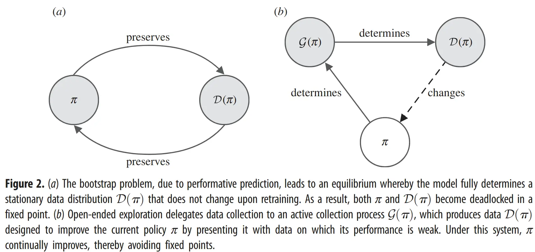
This dynamic is depicted in Figure 2a, where a model’s policy ($\pi$) shapes the data distribution ($\mathcal{D}(\pi )$) it sees, and retraining on this self-generated data simply preserves $\pi$, leading to a fixed, stagnant point:

Formalizing the Trap: Performative Prediction and Fixed Points

The bootstrap problem finds a more formal description in the concept of performative prediction. In this view, the model (with parameters $\theta$) actively influences the distribution of the training data $Z$, denoted as $\mathcal{D}(\theta )$, upon which it is subsequently trained. The critical issue arises from the system settling into an equilibrium, or a fixed point, between the model and the data distribution it shapes.

At such a fixed point, the model, now with parameters ${\theta }^{\ast }$, induces a data distribution $\mathcal{D}({\theta }^{\ast })$ that is identical to the very distribution it was last trained on to achieve ${\theta }^{\ast }$. These problematic fixed points, ${\theta }^{\ast }$, are defined as those satisfying the following equation:

$${\theta }^{\ast }=\arg \underset{\theta }{\min }{\mathbb{E}}_{Z\sim \mathcal{D}({\theta }^{\ast })}[\mathcal{L}(Z,\theta )]$$

Once at such a point, the online learning system effectively stagnates, its learning confined only to the data characteristics it currently generates, preventing any learning beyond this self-imposed boundary.

In effect, prioritized sampling in SL acts as a form of exploration, and RL's exploration methods can be seen as a form of prioritized sampling of experiences.

Transclude of exploration-vs-exploitation#^c914bd

Instead of viewing the problem as exploration from a single infinite MDP, it makes sense to think about the infinite space of MDPs, to emphasize and exploit the inherent modularity of the problem.

Criteria for high learning potential in automatic curriculum learning

E.g. exploring a subspace of environments: An MDP augmented with free parameters $\Theta$, where specifc configs $\theta$ are proposed by a teacher, its payoff $C:\Theta \to \mathbb{R}$ should adapt to the student’s capabilities, following the following criteria:

1. Improvability: The agent does not fully succeed. There is room for improvement.
2. Learnability: The agent can efficiently learn to improve.
3. Consistency: The solution to each environment configuration is consistent with those of other configurations.

“(iii) ensures that optimal behaviour in a proposed configuration does not conflict with that in another, e.g. entities are semantically consistent.”

Parametrized MDP ofc suffers all the same limitations. Can’t take shortcuts for open-endedness:

Open-ended exploration requires an open-ended simulation, one that continually expands to encompass new domains—in essence, exploring the space of possible MDPs.

Finally, the juicy part.

Exploring the full space of environments.

$\mathcal{G}(\pi )\to {\mathcal{D}}_{\mathcal{M}}$ … search process taking current policy and returning a distribution over the set of MDPs (a countably infinite set of programs under some turing-complete language).
By evaluating $\pi$ on $m\sim \mathcal{G}(\pi )$, we can iteratively update $\mathcal{G}(\pi )$ towards distributions over $\mathcal{M}$ that place greater weight on MDPs with higher learning potential, maximizing the learning potential criterion $C:\mathcal{M}\times \Pi \to \mathbb{R}$:

$$\begin{array}{r}{m}^{\ast }=\underset{m\in \mathcal{M}}{\mathrm{argmax}}C(m,\pi )\end{array}$$

$\mathcal{G}$ can consist of large parametric models alongside non-parametric models and human-in-the-loop components, and its components may shift over time.

When simply maximizing $C$ with a generative model, it might be intractable to even find a first valid MDP, let alone one that reflects problems of interest, and furthermore, it may trap the system in local optima of the first valid MDPs.
Hence, we begin the search near well-formed programs, reflecting tasks of interest:

$$\begin{array}{r}{m}^{\ast }=\arg \underset{m\in \mathcal{M}}{\max }\left(\underset{\text{learning potential}}{\underbrace{C(m,\pi )}}+{\alpha }_D\underset{\text{diversity}}{\underbrace{\sum _{m_i\in {\mathcal{M}}_Q}{\Delta }_D(m,m_i)}}-\underset{\text{grounding}}{\underbrace{\sum _{m_k\in {\mathcal{M}}_S}{\alpha }_k\cdot {\Delta }_G(m,m_k)}}\right)\end{array}$$

${\mathcal{M}}_S=\{m_k{\}}_{k=1}^K$ … target set of seed MDPS (paper uses $\bar{\mathcal{M}}$)
${\mathcal{M}}_Q$ … finite queue of top solutions found so far (paper uses $\hat{\mathcal{M}}$)
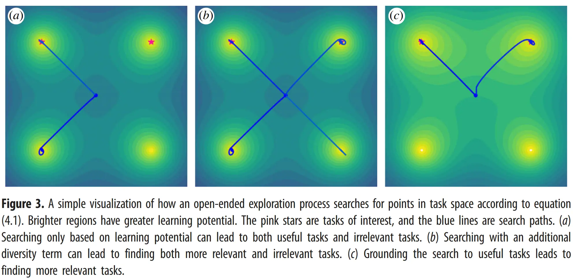
We maximizethe distance ${\Delta }_D$ between the current MDP and found solutions for diversity, and minimize the distance ${\Delta }_G$ to the seed MDPs for grounding.

${\Delta }_D,{\Delta }_G$ may use different notions of distance from eachother (string-edit distance, representation distance, …). ${\Delta }_G$ may encode inductive biases of what good MDPs look like (laws of physiscs, verifyable properties, …).

$M_S$ can be regularily updated to steer exploration toward specific regions in the space of MDPs (via humans/LLMs).

Distinction to quality diversity algorithms

Viewing the learning potential term as a measure of quality, we see that equation (4.2) implements a form of. However, this process remains significantly distinct from QD, as the measure of learning potential is a function of the current model, and therefore non-stationary throughout training. Moreover, learning potential is not transferable as a quality measure across agents in different training runs. To acknowledge the similarities to QD while highlighting its distinctness from QD, we call the problem of finding diverse data with high-learning potential that of learning-diversity.

Open-ended SL

We view a static SL dataset as aprametrized, single-step MDP (transition function $T$ terminates immediately) $m=(S=\{x_i{\}}_{i=1}^N,A=\mathcal{Y},\gamma =0,\rho =\mathcal{U}(S))$, with optimal policy $f$ that minimizes the emprical risk on $\mathcal{D}=\{(x_i,y_i){\}}_{i=1}^N$: ${\mathbb{E}}_{x_i\sim \rho }[\mathcal{L}(f(x_i),y_i)]$.
Selection functions of curriculum learning / active learning correspond to a specific $C(m,\pi )$, where $m$ now corrseponds to a datapoint in $D_{\text{train}}$, enabling open-ended exploration in SL:

More generally, as in RL, we can pursue the open-ended exploration criterion in SL through a combination of curating useful interaction data (i.e. online collection), manually collected seed datasets that reflect our domains of interest (i.e. offline collection), and actively generating data with high learning potential for our model using powerful generative models such as state-of-the-art diffusion models (?), grounded to these seed datasets.

Rant

Ooops this note is mostly copy pasta from the paper. Ig that’s because it’s a good and well-written paper … or lazy note taking? I mean it’s just well written and writing it down in my own words iss not worth the time right now, considering that half of it is somewhat obvious to me already, I just want the notes for future reference / summary / quick access because again, it’s presented in a good way, and rewriting just to have a 50% shorter, more to the point and memorable note, is not worth the extra hours it woulld take rn, esp with my broken index finger :sob: