Meta-Learning through Hebbian Plasticity in Random Networks

year: 2020
paper: https://arxiv.org/pdf/2007.02686.pdf
website:
code: https://github.com/enajx/HebbianMetaLearning
connections: ITU Copenhagen, meta learning, hebbian learning, lifelong learning, synaptic plasticity, adaptation, OpenAI-ES, generalization

---

Weights are plastic¹ according to the following hebbian rule learned for each synapse:

$$\Delta w_{ij}={\eta }_w\cdot (A_w{o}_i{o}_j+B_w{o}_i+C_w{o}_j+D_w)$$

where $o_i$ and $o_j$ are the pre- and post-synaptic activations, and ${\eta }_w,A_w,B_w,C_w,D_w$ are parameters learned through OpenAI-ES² during meta-training.
Networks are initialized with random weights, uniformly $\in [-0.1,01]$, adapting with each timestep (at meta-train and test time).

These networks can generalize to unseen morphologies, and recover from having a third of its weights set to zero, without any further training or reward signal.

Interestingly, the weights don’t converge to a stable configuration, but keep changing slightly during the agents lifetime.

Follow-up paper with real-world robots + improvements + …: Bio-Inspired Plastic Neural Networks for Zero-Shot Out-of-Distribution Generalization in Complex Animal-Inspired Robots

Potential future work: Introducing indirect encodings / revisiting previous work: Indirectly Encoding Neural Plasticity as a Pattern of Local Rules

---

In the case of the CarRacing environment the weights are normalised to the interval $[-1,+1]$, while the quadruped agents have unbounded weights.

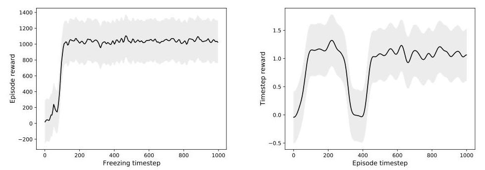
Left: The cumulative reward for the quadruped whose weights are frozen at different timesteps. The Hebbian network only needs in the order of 30–80 timesteps to converge to high-performing weights. Right: The performance of a quadruped whose actuators are frozen (saturating all its outputs to 1.0) during 100 timesteps (from t=300 to t=400). The robot is able to quickly recover from this perturbation in around 50 timesteps.

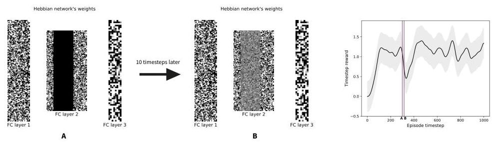
Resilience to weights perturbations. A: Visualisation of the network’s weights at the timestep when a third of its weights are zeroed out, shown as a black band. B: Visualisation of the network’s weights 10 timesteps after the zeroing; the network’s weights recovered from the perturbation. Right: Performance of the quadruped when we zero out a subset of the synaptic weights quickly recovers after an initial drop. The purple line indicates the timestep of the weight zeroing.

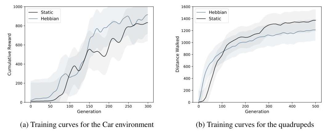
Even though the Hebbian method has to optimize a significant larger number of parameters, training performance increases similarly fast for both approaches.

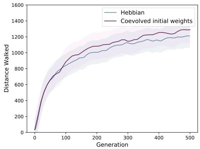
initializing the network with random weights at each episode and co-evolving the initial weights lead to similar results. Curves are averaged over three evolutionary runs.

---

Read the references of this par:

The most well-known form of synaptic plasticity occurring in biological spiking networks is spike- timing-dependent plasticity (STDP). On the other hand, artificial neural networks have continuous outputs which are usually interpreted as an abstraction of spiking networks in which the continuous output of each neuron represents a spike-rate coding average –instead of spike-timing coding– of a neuron over a long time window or, equivalent, of a subset of spiking neurons over a short time window; in this scenario, the relative timing of the pre and post-synaptic activity does not play a central role anymore [40, 41]. Spike-rate-dependent plasticity (SRDP) is a well documented phenomena in biological brains [42, 43]. We take inspiration from this work, showing that random networks combined with Hebbian learning can also enable more robust meta-learning approaches.

Mind blown. Had i known this + read the references 1yr ago, I’d’ve saved myself a few days of half baked research into stdp.

Footnotes

1. Weights of convolutional layers are static, only the FC layers are plastic. For convolutional filters, the concept of pre- and post-synaptic neurons is not well defined + “previous research on the human visual cortex indicates that the representation of visual stimuli in the early regions of the ventral stream are compatible with the representations of convolutional layers trained for image recognition”
   therefore suggesting that the variability of the parameters of convolutional layers should be limited.” ↩

2. black-box optimization methods have the benefit of not requiring the backpropagation of gradients and can deal with both sparse and dense reward

   ↩