Evolution Strategies as a Scalable Alternative to Reinforcement Learning

year: 2017
paper: Evolution Strategies as a Scalable Alternative to Reinforcement Learning
website: https://openai.com/index/evolution-strategies/
code: https://github.com/openai/evolution-strategies-starter | Karpathy gist | es-torch
connections: evolutionary optimization, RL, OpenAI, Illya Sutskever, natural evolution strategies, optimization

---

Evolution Strategies

Evolution Strategies (ES) is a class of black box optimization algorithms [Rechenberg and Eigen, 1973, Schwefel, 1977] that are heuristic search procedures inspired by natural evolution: At every iteration (“generation”), a population of parameter vectors (“genotypes”) is perturbed (“mutated”) and their objective function value (“fitness”) is evaluated. The highest scoring parameter vectors are then recombined to form the population for the next generation, and this procedure is iterated until the objective is fully optimized. Algorithms in this class differ in how they represent the population and how they perform mutation and recombination.

NES

This paper uses NES, where an objective function $F$ acting on parameters $\theta$ is optimized. What makes it a natural evolution strategy is that we arre not directly optimizing $\theta$, but optimizing a distribution over paramaters (“populations”) $p_{\psi }(\theta )$–itself parametrizd by $\psi$– and proceed to maximize the average objective value ${\mathbb{E}}_{\theta \sim p_{\psi }}F(\theta )$ over the population by searching for $\psi$ with stochastic gradient ascent, using the score function estimator for ${\nabla }_{\psi }{\mathbb{E}}_{\theta \sim p_{\psi }}F(\theta )$ similar to REINFORCE.
So gradient steps are taken on $\psi$ like this:

$$\begin{array}{r}{\nabla }_{\psi }{\mathbb{E}}_{\theta \sim p_{\psi }}F(\theta )={\mathbb{E}}_{\theta \sim p_{\psi }}\{F(\theta )\nabla \log p_{\psi }(\theta )\}\end{array}$$

We estimate the gradient by sampling the distribution because we can’t integrate over all possible values of $\theta$.
Their population distribution $p_{\psi }$ is a factored gaussian, the resulting gradient estimator is known as “simultaneous perturbation stochastic approximation”, “parameter-exploring policy gradients”, and “zero-order gradient estimation”.
The initial population distribution is an isotropic multivariate gaussian, with mean $\psi$ and fixed covariance ${\sigma }^{2}I$.
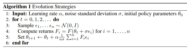
Initially, we optimize $\psi$ which controls a population distribution $p_{\psi }(\theta )$ that generates parameters $\theta$. However, by fixing $p_{\psi }$ as a Gaussian with mean $\theta$ and variance ${\sigma }^{2}I$, we can simplify this to directly optimizing $\theta$ by simply adding Gaussian noise $ϵ\sim N(0,I)$ during sampling. This transforms the problem from optimizing population distribution parameters ($\psi$) to directly optimizing the mean ($\theta$) of a fixed-form Gaussian, while maintaining exploration through noise injection. The resulting simplified gradient estimator:

$$\begin{array}{r}{\nabla }_{\theta }{\mathbb{E}}_{ϵ\sim N(0,I)}F(\theta +\sigma ϵ)=\frac{1}{\sigma }{\mathbb{E}}_{ϵ\sim N(0,I)}\{F(\theta +\sigma ϵ)ϵ\}\end{array}$$

This noise / gaussian blurring also allows us to train on non-differential / unsmooth environments.

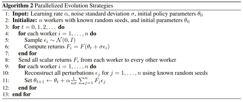
In parallel.

In the parallel version, the random seeds are fixed, such that the computation of parameter updates can happen on each worker independently, just the rewards need to be communicated. The duplicate operations (lines 9-12) are negligible.

One can imagine letting each worker only perturb a subset of parameters. $p_{\psi }$ → mixture of gaussians
With only one parameter change per worker → pure finite differences.

They say that not computing all the param updates on each worker would reduce computation in (9-12). But wouldn’t they have to communicate parameters again then?

When (not) to use ES?

TLDR: Depends strongly on the problem and monte-carlo estimator for gradients, but ES is better for long-horizon, long-lasting action effect, no good value-function available type problems (i.e. most things which are not games or toy problems).

We generally want a gradient estimator with lower variance:
High Variance → Need smaller learning rate → Slower learning
High Variance → Need more samples → More expensive training
High Variance → Less reliable updates → Potentially worse final performance

Assume correlation between reward and individual actions is low (as in any hard RL problem).
The variance of the gradient estimator (in this case simple monte-carlo, aka REINFORCE) for the two strategies is:

$$\begin{array}{rl}\text{Var}[\nabla F_{\text{PG}}(\theta )]& \approx \text{Var}[R(\mathbf{a})]\text{Var}[{\nabla }_{\theta }\log p(\mathbf{a};\theta )]\\ \text{Var}[\nabla F_{\text{ES}}(\theta )]& \approx \text{Var}[R(\mathbf{a})]\text{Var}[{\nabla }_{\theta }\log p(\tilde{\theta };\theta )]\end{array}$$

If both methods perform similar amounts of exploration, the variance from the reward term $\text{Var}[R(\mathbf{a})]$ will be similar.
The gradient for the policy-gradient method is ${\nabla }_{\theta }p(\mathbf{a};\theta )={\sum }_{t=1}^T{\nabla }_{\theta }\log p(a_t;\theta )$, a sum of $T$ uncorrelated terms, so its variance grows linearly with $T$ (the timesteps where an action is chosen in each).
The corresponding term for ES is ${\nabla }_{\theta }\log p(\tilde{\theta };\theta )$ has a variance is independent of $T$ because the noise in $\tilde{\theta }$ is independent of the timesteps → Better for long-horizon problems.

Policy Gradients variance $\propto T$; ES variance $\propto {\sigma }^2,\frac{1}{N}$

Variance in ES can be controlled by adjusting $\sigma$:
Smaller $\sigma$ → lower variance but might miss good directions
Larger $\sigma$ → higher variance but better exploration.
Or increasing the number of samples:
More samples → lower variance (by factor of $\frac{1}{N}$) but more computationally expensive

reward discounting reduces variance drastically, but is only applicable if actions have a short-lasting effect on the environment, else the gradients are biased.

Function approximation (for reducing the value of $T$) also runs the risk of biasing the gradients.

Variance methods used in this work.

“antithetic sampling” / “mirrored sampling”:
They always evaluate paris of perturbations $\pm ϵ$ for the gaussian noise-vector $ϵ$.
fitness shaping / applying a rank transformation to rewards:
To reduce the effect of outliers in the reward signal, applying a rank transformation means looking at their relative performance either like this [100,2,1]->[3,2,1] or normalized ranks like [1,.5,0].
This helps prevent premature convergence to local optima because one really good result pulls too strongly.

we did not see benefit from adapting $\sigma$ during training, and we therefore treat it as a fixed hyperparameter instead. We perform the optimization directly in parameter space; exploring indirect encodings (HyperNEAT, A Wavelet-based Encoding for Neuroevolution) is left for future work.

Are indirect encodings that promote regular structure like HyperNEAT good priors?

Transclude of indirect-encoding

Weight decay during training.

This prevents the parameters from growing very large compared to the perturbation — i.e. the noise is not drowned out by the parameters (no exploration).

ES can be seen as computing a finite difference derivative estimate in a randomly chosen direction, especially as $\sigma$ becomes small.

$${\nabla }_{\theta }F(\theta )={\mathbb{E}}_{ϵ\sim N(0,I)}\left\{F(\theta +\sigma ϵ)\frac{ϵ}{\sigma }\right\}={\mathbb{E}}_{ϵ\sim N(0,I)}\left\{(F(\theta +\sigma ϵ)-F(\theta ))\frac{ϵ}{\sigma }\right\}$$

This means, that for general non-smooth optimization problems, the required number of optimization steps scales linearly with the number of parameters $\theta$.

However, it is important to note that this does not mean that larger neural networks will perform worse than smaller networks when optimized using ES: what matters is the difficulty, or intrinsic dimension, of the optimization problem.

So something like approximating $y$ with $\hat{y}=xw$ does not become more difficult if we double the features and params by concatting $x$ with itself $x^{\prime }=(x,x)$. It will do exactly the same, as long as we divide the standard deviation of the noise by two, as well as the learning rate.
Why?
Because in this example, we’ve just represented the same problem in a higher dimensional space.
The adjustments need to be made because the noise sample vector is now twice as long, meaning the magnitude of the perturbation $\sigma ϵ$ would be larger just because there are more dimensions. The variance of from adding gaussian variables grows with the ​ of the number of dimensions.
The intrinsic difficulty of the problem stayed the same (think of it as talking a straight linein 2D vs 3D).
Of course the computational effort is still higher, but not the number of steps.
Just adding parameters does not make the optimization problem harder aka require you to do more steps, just if the additional parameters actually add to the problem.
In fact, bigger models are less prone to getting stuck in local optima.

Advantages of not calculating gradients.

By not requiring backpropagation, black box optimizers reduce the amount of computation per episode by about two thirds, and memory by potentially much more. In addition, not explicitly calculating an analytical gradient protects against problems with exploding gradients that are common when working with recurrent neural networks. By smoothing the cost function in parameter space, we reduce the pathological curvature that causes these problems: bounded cost functions that are smooth enough can’t have exploding gradients. At the extreme, ES allows us to incorporate non-differentiable elements into our architecture, such as modules that use hard attention.

Black box optimization methods are uniquely suited to low precision hardware for deep learning. Low precision arithmetic, such as in binary neural networks, can be performed much cheaper than at high precision. When optimizing such low precision architectures, biased low precision gradient estimates can be a problem when using gradient-based method.

By perturbing in parameter space instead of action space, black box optimizers are naturally invariant to the frequency at which our agent acts in the environment. For MDP-based reinforcement learning algorithms, on the other hand, it is well known that frameskip is a crucial parameter to get right for the optimization to succeed [Braylan et al., 2005]. While this is usually a solvable problem for games that only require short-term planning and action, it is a problem for learning longer term strategic behavior. For these problems, RL needs hierarchy to succeed [Parr and Russell, 1998], which is not as necessary when using black box optimization.

Paper comparing ES to PPO: Qualitative Differences Between Evolutionary Strategies and Reinforcement Learning Methods for Control of Autonomous Agents also introduces super-symmetric sampling, making the algorithm more efficient.

combine ES + UPGD + SSS?

Some optimizations for the current replica impl:

https://claude.ai/chat/7975f909-9f25-4bf7-a4da-6f9dcdff6c2e
Momentum? https://github.com/pytorch/pytorch/blob/b7bda236d18815052378c88081f64935427d7716/torch/optim/adam.py#L6
Improving Exploration in Evolution Strategies for Deep Reinforcement Learning via a Population of Novelty-Seeking Agents