reinforcement learning

Introduction to RL

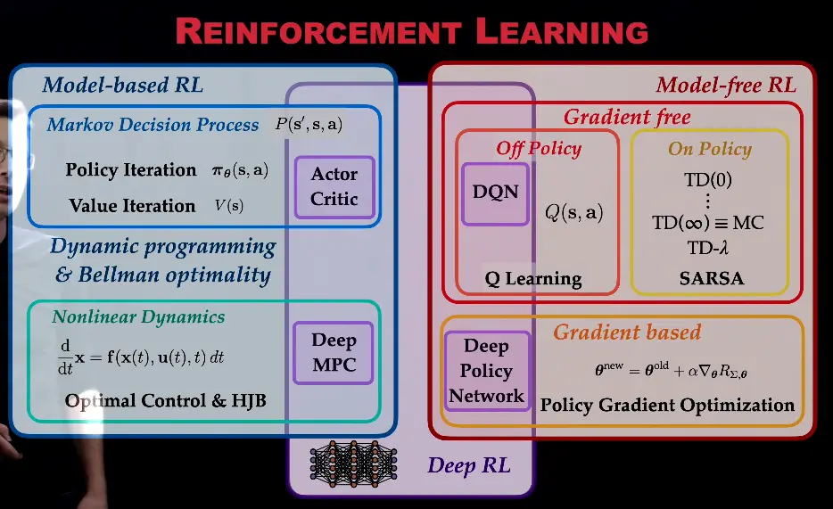
Intro from the neuroevolution book

RL takes many forms; the most dominant one has been based on Q-learning, i.e. the idea that different decisions at different states have different utility values (Q-values), which can be learned by comparing values available at successive states. An important aspect of such learning is that instead of storing the values explicitly as an array, a value function is learned that covers a continuous space of states and decisions. In that manner, the approach extends to large spaces often encountered in the real world. For instance, a humanoid robot can have many degrees of freedom, and therefore many physical configurations, and perform many different actions—even continuous ones. A value function assigns a utility to all combinations of them. This approach in particular has benefited from the progress in neural networks and deep learning, and the increase in available compute: it is possible to use them to learn more powerful value functions (e.g. DQN).
With sufficient compute, policy iteration has emerged as an alternative to Q-learning. Instead of values of decisions at states, the entire policy is learned directly as a neural network. That is, given a state, the network suggests an optimal action directly. Again, methods such as REINFORCE have existed for a long time (R. J. Williams, 1992), but they have become practical with modern compute.

monte carlo methods vs temporal difference learning vs dynamic programming

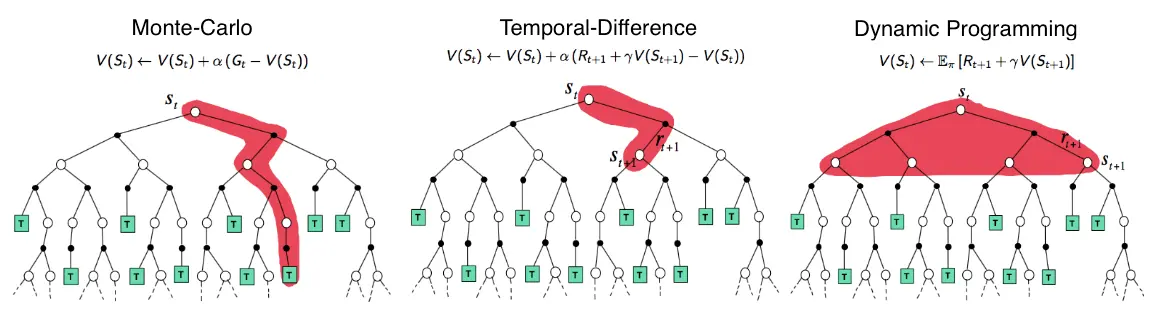
The picture shows the value propagation (“backup”) of a single update step with these three methods:

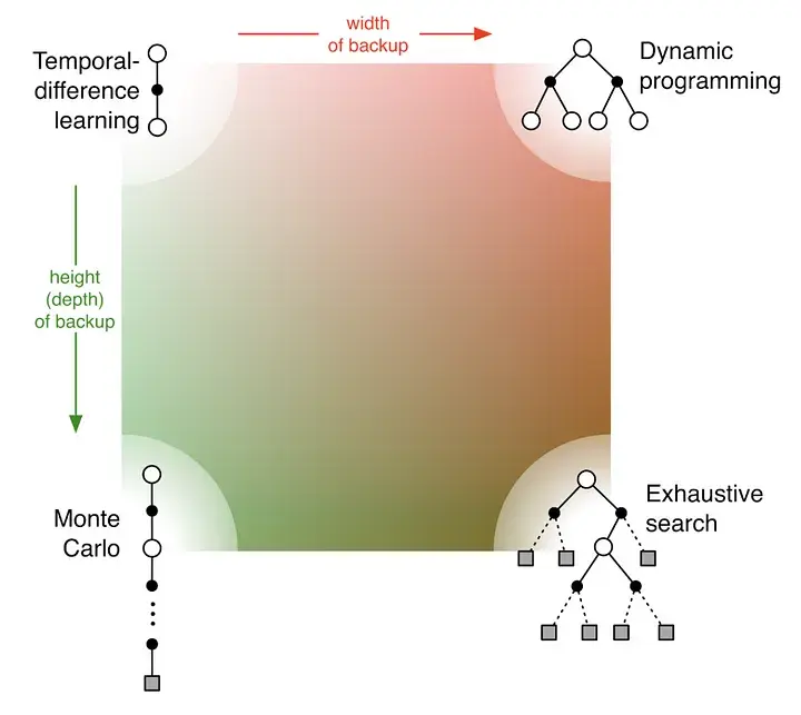
MC methods require complete episodes to learn, using actual returns $G_t$ to update value estimates. They’re unbiased (as long as there is exploration) but have high variance and require complete episodes (and thus more samples to achieve an accurate estimate, so bad for expensive environments), though truncated returns can also work.

TD bootstraps from existing value estimates after single steps, combining actual rewards with predicted future values. This introduces bias but reduces variance and enables online learning.

DP methods use the full model of the environment to consider all possible next states simultaneously, computing expected values directly. This is most sample-efficient (you don’t need to sample in order to approximate values – at the cost of exhaustive search) but requires a complete model of the environment, and are impractical for large state spaces, even with a perfect model (curse of dimensionality).

MC (left) vs TD

Types of policies

Deterministic policy: $a_t=\mu (s_t)$

Stochastic policy: $a_t\sim \pi (\cdot \mid s_t)$

Two major types are categorical policies for discrete action spaces and diagonal gaussian policies for continuous action spaces.

Categorical Policy

A categorical policy is just a classifier over discrete actions.
So like usual you have feature extraction → logits → softmax → sample an action.
Get the log-likelihood for the action $a$ at state $s$ by indexing the log of the output vector: $\log {\pi }_{\theta }(a|s)$.

Diagonal Gaussian Policy

Diagonal gaussian policies map from observations to mean actions ${\mu }_{\theta }(s)$.
There’s two common ways to represent represent the covariance matrix:

A parameter vector of log standard deviations $\log {\sigma }_{\theta }$, which is not a function of state.

Network layers mapping from states to log standard deviations $\log {\sigma }_{\theta }(s)$, may share params with ${\mu }_{\theta }$.

We can then just sample from the distribution to get an action.

Log standard deviations are used so we don’t have to constrain the ANN output to be nonnegative, and can simply exponentiate the log outputs to obtain $\sigma$, without loosing anything.

Link to original

Limitations of RL

From General intelligence requires rethinking exploration:
As RL agents train on their own experiences, locally optimal behaviours can easily self-reinforce, preventing the agent from reaching better optima. To avoid such outcomes and ensure sufficient coverage of possible MDP transitions during training, RL considers exploration a principal aim.

Under exploration, the RL agent performs actions in order to maximize some measure of novelty of the resulting experiential data or uncertainty in outcome, rather than to maximize return (ICM, CEED. Simpler still, new and informative states can often be unlocked by injecting noise into the policy, e.g. by sporadically sampling actions uniformly at random (see epsilon greedy, PPO). However, such random search strategies (also ES) can run into the curse of dimensionality, becoming less sample efficient in practice.

A prominent limitation of state-of-the-art RL methods is their need for large amounts of data to learn optimal policies. This sample inefficiency is often attributable to the sparse reward nature of many RL environments, where the agent only receives a reward signal upon performing some desired behaviour. Even in a dense reward setting, the agent may likewise see sample-inefficient learning once trapped in a local optimum, as discovering pockets of higher reward can be akin to finding a similarly sparse signal.

In complex real-world domains with large state spaces and highly branching trajectories, finding the optimal behaviour may require an astronomical number of environment interactions, despite performing exploration. Thus for many tasks, training an RL agent using real-world interactions is highly costly, if not completely infeasible. Moreover, a poorly trained embodied agent acting in real-world environments can potentially perform unsafe interactions. For these reasons, RL is typically performed within a simulator, with which massive parallelization can achieve billions of samples within a few hours of training.
Simulation frees RL from the constraints of real-world training at the cost of the sim2real gap, the difference between the experiences available in the simulator and those in reality. When the sim2real gap is high, RL agents perform poorly in the real world, despite succeeding in simulation. Importantly, a simulator that only implements a single task or small variations thereof will not produce agents that transfer to the countless tasks of interest for general intelligence. Thus, RL ultimately runs into a similar data limitation as in SL.
In fact, the situation may be orders of magnitude worse for RL, where unlike in SL, we have not witnessed results supporting a power-law scaling of test loss on new tasks, as a function of the amount of training data. Existing static RL simulators may thus impose a more severe data limitation than static datasets, which have been shown capable of inducing strong generalization performance.

---

From neuroevolution book:

Importantly, however, scale-up is still an issue with RL. Even though multiple modifications can be evaluated in parallel and offline, the methods are still primarily based on improving a single solution, i.e. on hill-climbing. Creativity and exploration are thus limited. Drastically different, novel solutions are unlikely to be found because the approach simply does not explore the space widely enough. Progress is slow if the search landscape is high-dimensional and nonlinear enough, making it difficult to find good combinations. Deceptive landscapes are difficult to deal with since hill-climbing is likely to get stuck in local minima. Care must thus be taken to design the problem well so that RL can be effective, which also limits the creativity that can be achieved.

While IRL, organisms receive intrinsic rewards, in contemporary RL this is turned on its head: The agent receives extrinsic rewards from the environment, which tells it what’s good and what’s bad. If we want to create agentic, open-ended AI / ALIFE, we should think about how to make them intrinsically motivated.

Best paper I’ve read all year (‘24) on this: Embracing curiosity eliminates the exploration-exploitation dilemma.

---

messy old notes below

RL is useful if you want to adjust your world model while you are operating in the real world. The way to adjust your world model for the situation at hand is to explore parts of the space where the world model is inaccurate → curiosity / play.

Difficulties in RL with data: ¹

• non-stationary (changing distribution)
• depends on your model
• credit assignment (unclear which actions was good)
  Stuff that makes or breaks trainings in practice:
• keeping state/state-action values in a reasonable range (equation 3.10 in Sutton & Barto can help you upper bound the magnitudes, an upper bound on the order of 1e1 usually works for me)
• balancing exploration and exploitation right
• effective learning rates - the value of n in n-step returns (5 to 20 is usually good)

Danie Hafner (YT):
Deep Hierarchical Planning from Pixels
Dream to Control: Learning Behaviors by Latent Imagination
v2

---

Introduction to RL

Deep Reinforcement Learning: Pong from Pixels
Lessons Learned Reproducing a Deep Reinforcement Learning Paper
https://lilianweng.github.io/posts/2018-02-19-rl-overview/

Types of RL

https://www.reddit.com/r/reinforcementlearning/comments/utnhia/what_is_offline_reinforcement_learning/?rdt=45931
Offline Reinforcement Learning: Tutorial, Review, and Perspectives on Open Problems

online learning
off-policy
on-policy

Resources

Intro

• First, you want to fresh up on probability.
• Steve brunton RL
• https://spinningup.openai.com/en/latest/user/introduction.html / gh
• reinforcement learning book
  • https://towardsdatascience.com/introduction-to-reinforcement-learning-rl-part-6-temporal-difference-td-learning-2a12f0aba9f9

Code

• minimal RL
• CleanRL: Code for popular RL algs

stable-baselines blog is good (contains only policy gradients) but papers are the best resource.
policy gradients : https://stable-baselines3.readthedocs.io/en/master/guide/algos.html, using ssl and data augmentation along with policy gradients, Dreamer and other world models, Decision Transformer, and many more.
The book got boring after some chapters so i just implemented papers from this blog and it’s references https://lilianweng.github.io/posts/2018-02-19-rl-overview/

Environments

CRAFTAX

• gymnasium
• pufferlib (prlly not as useful to us, but is a communication layer with which you can use policies etc. neatly with many RL envs together)
  • Neural MMO
• https://github.com/chernyadev/bigym Demo-Driven Mobile Bi-Manual Manipulation Benchmark.

Footnotes

1. George Hotz | Researching | RL is dumb and doesn’t work (theory) | Reinforcement Learning | Part 3) ↩