year: 2024/08
paper: https://www.nature.com/articles/s41586-024-07711-7
website:
code:
connections: loss of plasticity, continual learning, Richard Sutton, AMII, continual backpropagation, backpropagation, deep learning
Takeaways
→ Backprop is plastic, but only in the beginning (see Why does backprop loose plasticity?).
→ Small weights reduce loss of plasticity.
→ Continual injection of variability mitigates loss of plasticity.
→ Loss of plasticity is most relevant for systems that use small or no replay buffers, as large buffers can hide the effect of new data. Overcoming loss of plasticity is an important step towards deep reinforcement-learning systems that can learn from an online data stream.
→ deep learning is an effective and valuable technology in settings in which learning occurs in a special training phase and not thereafter. In settings in which learning must continue, however, we have shown that deep learning does not work. By deep learning, we mean the existing standard algorithms for learning in multilayer artificial neural networks and by not work, we mean that, over time, they fail to learn appreciably better than shallow networks.
→ Although Shrink and Perturb adds variability / injects noise to all weights, continual backpropagation does so selectively, and this enables it to better maintain plasticity - by effectively removing all dead units (→ higher effective rank; + less sensitive to hparams than S&P). Continual backpropagation involves a form of variation and selection in the space of neuron-like units, combined with continuing gradient descent. The variation and selection is reminiscent of trial-and-error processes in evolution and behaviour (as opposed to just following gradient ig).
→ Dropout, batch normalization/online normalization, and Adam also seems to reduce plasticity, though the paper did not investigate why. In general - these standard methods improve performance initially / on a static distribution, but are terrible for continual learning (or RL for that matter, as the policy is also ever changing - so much so, that periodically reinitializing network weights is better than keeping the trained one… provided there is a large buffer - else everrything would be forgotten).
→ Plasticity (adapting) != stability (memorizing; catastrophic forgetting). The utility in continual BP in its current form only tackles plasticity.
Why does backprop loose plasticity?
The only difference in the learner over time is the network weights. In the beginning, the weights were small random numbers, as they were sampled from the initial distribution; however, after learning some tasks, the weights become optimized for the most recent task. Thus, the starting weights for the next task are qualitatively different from those for the first task. As this difference in the weights is the only difference in the learning algorithm over time, the initial weight distribution must have some unique properties that make backpropagation plastic in the beginning. The initial random distribution might have many properties that enable plasticity, such as the diversity of units, non-saturated units, small weight magnitude etc.
Three phenomena that correlate with - and partially explain - the loss of plasticity:
→ Increase of dead units.
→ Higher weight magnitude (corresponds to worse learning/performance - due to sharper curvature, see hessian).
→ Drop in effective rank of hidden layers, i.e. redundancy/low utility of many units for the layer output.However, a low-rank solution might be a bad starting point for learning from new observations because most of the hidden units provide little to no information. The decrease in effective rank could explain the loss of plasticity in our experiments in the following way. After each task, the learning algorithm finds a low-rank solution for the current task, which then serves as the initialization for the next task. As the process continues, the effective rank of the representation layer keeps decreasing after each task, limiting the number of solutions that the network can represent immediately at the start of each new task.
Link to originalIs continual backprop ~= UPGD, just that they measure utility a little differently?
→ Indeed it is - UPGD is a better version - from the UPGD paper:
The generate-and-test method (Mahmood & Sutton 2013) is a method that finds better features using search, which, when combined with gradient descent (see Dohare et al. 2023a), is similar to a feature-wise variation of our method. However, this method only works with networks with single-hidden layers in single-output regression problems. It uses the weight magnitude to determine, such as classification (Elsayed 2022). On the contrary, our variation uses a better notion of utility that enables better search in the feature space and works with arbitrary network structures or objective functions so that it can be seen as a generalization of the generate-and-test method.
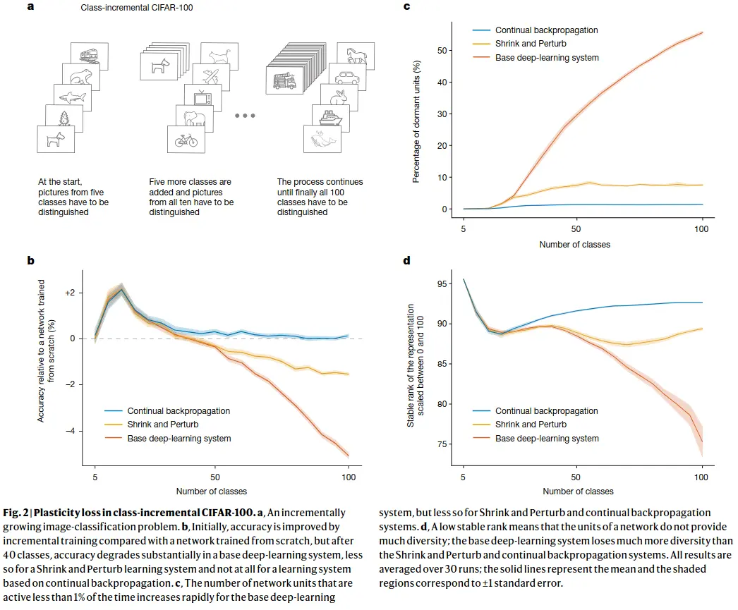
Class-incremental continual learning
… involves sequentially adding new classes while testing on all classes seen so far. In our demonstration, we started with training on five classes and then successively added more, five at a time, until all 100 were available. After each addition, the networks were trained and performance was measured on all available classes. We continued training on the old classes (unlike in most work in class-incremental learning) to focus on plasticity rather than on forgetting.
…
As more classes are added, correctly classifying images becomes more difficult and classification accuracy would decrease even if the network maintained its ability to learn. To factor out this effect, we compare the accuracy of our incrementally trained networks with networks that were retrained from scratch on the same subset of classes. For example, the network that was trained first on five classes, and then on all ten classes, is compared with a network retrained from scratch on all ten classes. If the incrementally trained network performs better than a network retrained from scratch, then there is a benefit owing to training on previous classes, and if it performs worse, then there is genuine loss of plasticity.
Two baselines:
A) Base neural network: A18-layer resnet, with warmup, batch norm, data augmentation and L2 regularization.
B) Base net with the “shrink and perturb” algorithm, where the weights of the network are multiplied by a constant , and small random noise sampled from a normal distribution is added at the start of each new phase (new classes being added), so the new weights are: .
Experiments
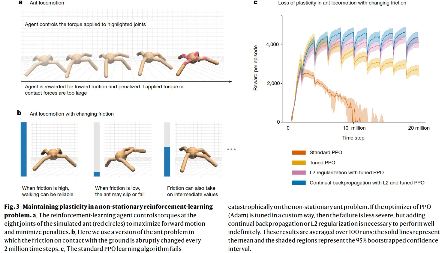
Continual backprop performs well even if RL episodes go on for longer or if new tasks are added - old information is beneficial or at least not detrimental, whereas for regular backprop, or even backprop with L2 regularization or with the shrink and perturb algorithm, training a net from scratch is better than using the old one! (though shrink and perturb and L2 reg help massively)
Continual backprop
Continual backpropagation selectively reinitializes low-utility units in the network. Our utility measure, called the contribution utility, is defined for each connection or weight and each unit. The basic intuition behind the contribution utility is that the magnitude of the product of units’ activation and outgoing weight gives information about how valuable this connection is to its consumers. If the contribution of a hidden unit to its consumer is small, its contribution can be overwhelmed by contributions from other hidden units. In such a case, the hidden unit is not useful to its consumer. We define the contribution utility of a hidden unit as the sum of the utilities of all its outgoing connections. The contribution utility is measured as a running average of instantaneous contributions with a decay rate , which is set to in all experiments. in a feed-forward neural network, the contribution utility, , of the hidden unit in layer at time is updated as:
\boldsymbol{u}{l}[i] = \eta \cdot\boldsymbol{u}{l}[i] + (1 - \eta) \cdot |\boldsymbol{h}{l,i,t}| \cdot\sum^{n{l+1}}{k=1} |\boldsymbol{w{l,i,k,t}}|
… where $\boldsymbol{h}_{l,i,t}$ is the output of the $i^{\text{th}}$ hidden unit in layer $l$ at time $t$, $\boldsymbol{w}_{l,i,k,t}$ is the weight connecting the $i^{\text{th}}$ unit in layer $l$ to the $k^{\text{th}}$ unit in layer $l+1$ at time $t$, and $n_{l+1}$ is the number of units in layer $l+1$. However, initializing the outgoing weight to zero makes the new unit vulnerable to immediate reinitialization, as it has zero utility. To protect new units from immediate reinitialization, they are protected from a reinitialization for maturity threshold $m$ number of updates. We call a unit mature if its age is more than $m$. Every step, a fraction of mature units $\rho$, called the replacement rate, is reinitialized in every layer. The replacement rate is typically set to a very small value, meaning that only one unit is replaced after hundreds of updates.