expected value

$\mathbb{E}$ stands for the expectation, which is a mathematical operator that calculates the average value of a random variable over many possible outcomes.

In short, it’s the mean/“center of mass” of a probability distribution

$$\mu =\mathbb{E}\left[X\right]=\sum _{i=1}^{n}P(X=x_i)\cdot x_i$$

$X\dots$ random variable (distribution), can be discrete or continuous
$x_i\dots$ possible outcomes of the random variable $X$
The expected value of a random variable is like saying you go through all of the possible outcomes and multiply the probability of that outcome times the value of that variable (weighted average).

For continous random variables (described by PDFs), the expected value is:

$$\mathbb{E}[X]={\int }_{-\infty }^{\infty }x\cdot f(x)dx$$

The integral exetends over all possible values of $X$.
In a more general notation:

$$\mathbb{E}[g(X)]={\int }_{x}f(x)g(x)$$

where $f(x)$ is the probability density function and $g(x)$ is the expectation function of the random variable and ${\int }_x$ is shorthand for integrating over all possible values of $X$.

Expectations can be approximated by with a sample mean:

$$\mathbb{E}[X]\approx \frac{1}{n}\sum _{i=1}^n{x}_i$$ $$\underset{n\to \infty }{\lim }\frac{1}{n}\sum _{i=1}^n{x}_i\to \mu =\mathbb{E}[X]$$

If we draw from a particular distribution $P$, we write it like this

$$\underset{x\sim P}{\mathbb{E}}[X]={\int }_{x}P(x)x$$

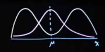
For oddly shaped distributions, the expected value might not actually correspond ot a common value in the distribution

The gaussian and bimodal distributions below have the same $\mu$, but the bimodal distribution almost never takes on that value:

Properties

The expected value is linear

$$\begin{array}{r}\mathbb{E}[X+Y]=\mathbb{E}[X]+\mathbb{E}[Y]\end{array}$$

The expected value is a constant and constants stay constants

$$\begin{array}{rl}\mathbb{E}[\mathbb{E}[X]]& =\mathbb{E}[X]\\ \mathbb{E}[X+c]& =\mathbb{E}[X]+c\\ \mathbb{E}[cX]& =c\mathbb{E}[X]\end{array}$$

If the distribution is uniform, the expected value simplifies to the arithmetic mean of the values.

Only if $X,Y$ are independent, then …

$$\mathbb{E}[XY]=\mathbb{E}[X]\cdot \mathbb{E}[Y]$$

Derivation

\begin{align*}
\mathbb{E}(XY) &= \sum_{x} \sum_{y} xy , \underbrace{ P(X=x, Y=y) }{ \text{if independent} } \
&= \sum{x} \sum_{y} xy , P(X=x) P(Y=y) \
&= \left(\sum_{x} x , P(X=x)\right) \left(\sum_{y} y , P(Y=y)\right) \
&= \mathbb{E}[X] \cdot \mathbb{E}[Y]
\end{align*}

Where/Why it doesn’t hold $\mathbb{E}[XY]\ne \mathbb{E}[X]\mathbb{E}[Y]$ because the joint distribution $P(X,Y)\ne P(X)P(Y)$. The difference is captured by the covariance: $\text{Cov}(X,Y)=\mathbb{E}[XY]-\mathbb{E}[X]\mathbb{E}[Y]$

For dependent variables,

Parent-child height $X$ = parent height, $Y$ = child height Parents: 160, 180 → $\mathbb{E}[X]=170$ Children: 155, 175 → $\mathbb{E}[Y]=165$
Joint pairs: (160,155), (180,175) $\mathbb{E}[X]\mathbb{E}[Y]=170\times 165=28,050$ $\mathbb{E}[XY]=\frac{160\times 155+180\times 175}{2}=\frac{24,800+31,500}{2}=28,150$ The positive correlation ($\text{Cov}=100$) makes tall$\times$tall and short$\times$short pairs more likely, increasing $\mathbb{E}[XY]$ above the independent case.

Let

Law of the Unconscious Statistician (LOTUS)

For $Y=g(X)$, you can compute $E[Y]$ directly using $X$‘s distribution:

\begin{align*} E[g(X)] = \cases{ \sum_{x} g(x) P(x) & \text{discrete} \cr \int_{-\infty}^{\infty} g(x) f(x) \, dx & \text{continuous} } \end{align*}

Important: $E[g(X)]\ne g(E[X])$ in general (only equal for linear functions)

$X\in \{0,2\}$ with $P(X=0)=P(X=2)=0.5,g(x)=x^2$ $E[X]=1$, $g(E[X])=1^2=1$, but $E[X^2]=0.5(0^2)+0.5(2^2)=2$

Let

Common notations for expectations

$\mathbb{E}[f(X)]$ — after declaring $X\sim P$. (Very common in stats/prob.)
${\mathbb{E}}_X[f(X)]$ or ${\mathbb{E}}_x[f(x)]$ — variable-centric.
${\mathbb{E}}_P[f(X)]$ — measure/distribution-centric. (Favored in info theory; clean when $f$ doesn’t name $x$.)
${\mathbb{E}}_{x\sim P}[f(x)]$ — explicit sampling form. (Very common in ML.)
${\mathbb{E}}_p[f(X)]$ or ${\mathbb{E}}_{x\sim p(x)}[f(x)]$ — when referring to a density $p$.
$\int f\mathrm{d}P$, $\int f(x)p(x)\mathrm{d}x$, ${\sum }_{x}f(x)p(x)$ — measure/integral form. (Probability/info theory texts.)
$⟨f(X){⟩}_P$ — physics/stat-mech style; you’ll sometimes see it in evolutionary/EC papers.
Parametric models: ${\mathbb{E}}_{P_{\theta }}[f(X)]$ or ${\mathbb{E}}_{p_{\theta }}[f(X)]$, sometimes ${\mathbb{E}}_{\theta }[\cdot ]$.
Machine learning (incl. VI/RL): ${\mathbb{E}}_{x\sim p_{\text{data}}}[\cdot ]$, ${\mathbb{E}}_{z\sim q_{\varphi }}[\cdot ]$; Monte Carlo $\frac{1}{n}{\sum }_i$.

---

Converting Celius to Fahrenheit $\mathbb{E}[aX+b]$ & $\text{Var}(aX+b)$

I measure $X$ in ${}^{\circ }C$, and want the expected value and variance in ${}^{\circ }F$, $a=\frac{9}{5},b=32$. $Y=ax+b$

$$\begin{array}{rl}\mathbb{E}[Y]=\mathbb{E}[aX+b]& =\int (ax+b)f(x)dx\text{LOTUS}\\ & =\int axf(x)dx+\int bf(x)dx\\ & =a\underset{\mathbb{E}[x]}{\underbrace{\int xf(x)dx}}+b\underset{1}{\underbrace{\int f(x)dx}}\\ & =a\mathbb{E}[X]+b\end{array}$$

→ Since $Y$ is a linear function of $X$, we can directly transform the expectation.

---

$$\begin{array}{rl}\text{Var}(aX+b)=\text{Var}(Y)& =\mathbb{E}[(Y-\mathbb{E}[Y{]}^2)]\\ & =\mathbb{E}[(aX\cancel{+b}-a\mathbb{E}[X]\cancel{-b}]{)}^2]\\ & =\mathbb{E}[a^2-(X-\mathbb{E}[X]{)}^2]\\ & =a^2\mathbb{E}[(X-\mathbb{E}[X]{)}^2]\\ & =a^2\text{Var}(X)\end{array}$$

→ Variance changes with change of units / scale, but is not affected by shifts.

Tail Sum Formula

For a non-negative random variable $X\in \{0,\dots ,n\}$, the expected value can be computed using the tail sum formula:

$$\begin{array}{rl}\mathbb{E}[X]& =\sum _{k=1}^{n}P(X\ge k)\\ & =\sum _{k=0}^{n}kP(X=k)\\ & =1p_1+2p_2+3p_3+\cdots +(n-1)p_{n-1}+n{p}_n\\ & =\{\begin{array}{l}P(X\ge 1)\\ +P(X\ge 2)\\ +P(X\ge 3)\\ +\cdots \\ +P(X\ge n-1)\\ +P(X\ge n)\end{array}\begin{array}{l}=p_1+p_2+p_3+\cdots +p_n\\ +p_2+p_3+\cdots +p_n\\ +p_3+\cdots +p_n\\ +\cdots \\ +p_{n-1}+p_n\\ +p_n\end{array}\end{array}$$

Note that $P(X\ge k)=1-P(X\le k)=1-F_X(k)$, where $F_X$ is the cumulative distribution function of $X$.

Link to original

References

https://chat.openai.com/c/92cd3571-92b1-4c8f-8345-b62a753888e3

probability