monte carlo method

Monte Carlo Gradient Estimation in Machine Learning

year: 2020
paper: https://arxiv.org/pdf/1906.10652
website:
code:
connections: monte carlo method, machine learning

---

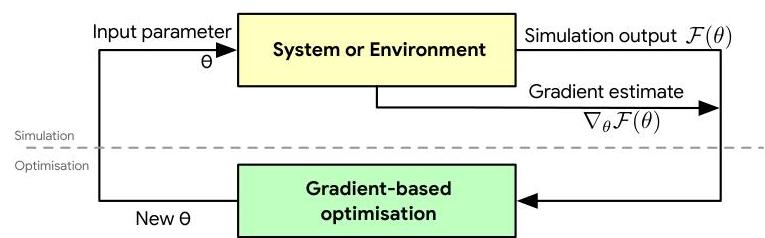
Whereas in a typical optimisation we would make a call to the system for a function value, which is deterministic, in stochastic optimization we make a call for an estimate of the function value; instead of calling for the gradient, we ask for an estimate of the gradient; instead of calling for the Hessian, we will ask for an estimate of the Hessian; all these estimates are random variables.

Problem statement

$\mathcal{F}$ is a probabilistic objective of the form:

$$\begin{array}{r}\mathcal{F}(\theta ):=\int p_{\mathbf{\theta }}(x)f_{\mathbf{\varphi }}(x)dx={\mathbb{E}}_{p_{\mathbf{\theta }}(x)}[f_{\mathbf{\varphi }}(x)]\end{array}$$

where $f$ is a function of an input variable $x$ with “structural parameters” $\varphi$, evaluated on average with respect to the input distribution $p_{\mathbf{\theta }}(x)$ with distributional parameters $\mathbf{\theta }$.
$f$ is referred to as cost and $p_{\mathbf{\theta }}$ as measure ¹. They call this a “mean-value analysis”.

→ This is a general framework that allows us to cover problems from queueing theory and variational inference to portfolio design and reinforcement learning.

We want to learn $\mathbf{\theta }$ by optimizing $\mathcal{F}(\theta )$, so we care about its gradient:

$$\mathbf{\eta }:={\nabla }_{\mathbf{\theta }}\mathcal{F}(\mathbf{\theta })={\nabla }_{\mathbf{\theta }}{\mathbb{E}}_{p_{\mathbf{\theta }}(x)}[f_{\mathbf{\varphi }}(x)]$$

They call this the “sensitivity analysis” of $\mathcal{F}$ , i.e. the gradient of the expectation with respect to the distribution parameters $\mathbf{\theta }$. It characterizes the behavior of the costs’s sensitivity to changes in the distribution parameters. ²³

→ This gradient lies at the core of tools for model explanation [probabilistic systems] and optimisation.
But this gradient problem is difficult in general: we will often not be able to evaluate the expectation in closed form; the integrals over $x$ are typically high-dimensional making quadrature ineffective; it is common to request gradients with respect to high-dimensional parameters $\theta$, easily in the order of tens-of-thousands of dimensions; and in the most general cases, the cost function may itself not be differentiable, or be a black-box function whose output is all we are able to observe. In addition, for applications in machine learning, we will need efficient, accurate and parallelisable solutions that minimise the number of evaluations of the cost. These are all challenges we can overcome by developing Monte Carlo estimators of these integrals and gradients,

$\varphi$ is not considered in the following ($\varphi$ shapes how each sampled $x$ is scored, but don’t affect how it is sampled, in this setup) which is why the paper drops it, even though may depend on it.

Monte Carlo estimator of the expectation $\mathcal{F}(\theta )$

The monte carlo method lets us approximate the estimation in cases where we can’t (easily) evaluate the integral in closed form, by drawing iid samples ${\hat{x}}^1,\dots ,{\hat{x}}^{(N)}$ from the distribution $p_{\theta }(x)$, and taking the average of the function evaluated at those samples:

$${\bar{\mathcal{F}}}_N=\frac{1}{N}\sum _{n=1}^{N}f({\hat{x}}^{(n)}),\text{where }{\hat{x}}^{(n)}\sim p_{\mathbf{\theta }}(x)\text{ for }n=1,\dots ,N$$

I.e. we approximate the expectation by the empircal/sample mean of $N$ samples.
All we need is an integral of the form shown above, and a distribution that we can easily sample from.

The resulting quantity ${\bar{\mathcal{F}}}_N$ is a random variable, because it deends on the set of random variates used.

Desirable properties of Monte Carlo estimators:

Consistency

The estimator should converge to the true value as the number of samples increases:

\bar{\mathcal{F}}_{N} \xrightarrow{a.s.} \mathcal{F}(\theta) \text{ as } N \to \infty

Following the strong law of large numbers.

Un biasedness The estimate of the gradient should be correct on average. Unbiasedness is always preferred because it allows us to guarantee the convergence of a stochastic optimization procedure.

\mathbb{E}{p{\theta}(x)}[\bar{\mathcal{F}}_{N}] = \mathcal{F}(\theta)

This follows from the linearity of expectation and the fact that the samples are drawn from $p_{\theta }(x)$:

\begin{align*}
\mathbb{E}{p{\theta}(x)}[\bar{\mathcal{F}}{N}] &= \mathbb{E}{p_{\theta}(x)}\left[\frac{1}{N} \sum_{n=1}^{N}f(\hat{x}^{(n)})\right] \
&= \frac{1}{N} \sum_{n=1}^{N} \mathbb{E}{p{\theta}(x)}[f(\hat{x}^{(n)})] \
&= \frac{1}{N} \sum_{n=1}^{N} \mathcal{F}(\theta) \
&= \mathcal{F}(\theta)
\end{align*}

Minimum variance. Evolution Strategies as a Scalable Alternative to Reinforcement Learning also makes good points about variance reduction.

Comparing two unbiased estimators, the one with lower variance is better.
Low-variance gradients allow larger learning rates (→ fewer steps) and more stable convergence.

Computational efficiency

Less evaluations/samples (linear cost in the number of parameters) + parallelizable = good.

Making a clear separation between the simulation and optimisation phases allows us to focus our attention on developing the best estimators of gradients we can, knowing that when used with gradient-based optimisation methods available to us, we can guarantee convergence so long as the estimate is unbiased, i.e. the estimate of the gradient is correct on average.

Sources of stochasticity:

• environment
• (optionally) SGD (sampling minibatches)

The Bias-Variance Tradeoff Different gradient estimators (score function, pathwise, etc.) have different bias-variance properties.
Score function is unbiased but high variance. Pathwise (reparameterization) has lower variance but requires differentiable f(x).

Example applications:

Variational Inference

Variational inference

Variational inference is a general method for approximating complex and unknown distributions by the closest distribution within a tractable family. Wherever the need to approximate distributions appears in machine learning—in supervised, unsupervised, reinforcement learning—a form of variational inference can be used.

Consider a generic probabilistic model $p(x|z)p(z)$ that defines a generative process in which observed data $x$ is generated from a set of unobserved variables $z$ using a a data distribution $p(x|z)$ and a prior distribution $p(z)$.
In supervised learning, the unobserved variables might correspond to the weights of a regression problem, and in unsupervised learning to latent variables.
The posterior distribution of this generative process $p(z|x)$ is unknown, and is approximated by a variational distribution $q(z|x;\mathbf{\theta })$, which is a parameterised family of distributions with variational parameters $\mathbf{\theta }$, e.g., the mean and variance of a gaussian distribution. Finding the distribution $q(z|x;\mathbf{\theta })$ that is closest to $p(z|x)$ (e.g. in the KL sense) leads to an objective, the variational free energy, that optimizes an expected log-likelihood $\log p(x|z)$ subject to a regularization constraint that encourages closeness between the variational distribution $q$ and the prior distribution $p(z)$.

Optimising the distribution $q$ requires the gradient of the free energy with respect to the variational parameters $\mathbf{\theta }$:

$$\begin{array}{rl}\mathbf{\eta }& ={\nabla }_{\mathbf{\theta }}{\mathbb{E}}_{q(z|x;\mathbf{\theta })}\left[\log p(x|z)-\log \frac{q(z|x;\mathbf{\theta })}{p(z)}\right]\end{array}$$

This is an objective in the form we have in monte carlo estimation, where the cost function is the term in square brackets, and the measure is the variational distribution $q(z|x;\mathbf{\theta })$.

This problem also appears in other research areas, especially in statistical physics, information theory and utility theory. Many of the solutions that have been developed for scene understanding, representation learning, photo-realistic image generation, or the simulation of molecular structures also rely on variational inference.

Link to original

Reinforcement Learning

Policy gradient methods

Let $s_0$ be sampled from initial distribution ${\rho }_0$. A trajectory $(s_0,a_0,s_1,a_1,\dots )$ is generated by:

• Sampling actions: $a_t\sim \pi (a_t\mid s_t)$
• Sampling states: $s_{t+1}\sim P(s_{t+1}\mid s_t,a_t)$

until reaching a terminal state. At each timestep, a reward $r_t=r(s_t,a_t,s_{t+1})$ is received. The goal is to maximize the expected total reward ${\sum }_{t=0}^{\infty }{r}_t$ (assumed to be finite).

Policy gradient methods maximize the expected total reward by estimating the gradient $g$:

$$g:={\nabla }_{\theta }{\mathbb{E}}_{{\pi }_{\theta }}\left[\sum _{t=0}^{\infty }{r}_t\right]\approx \mathbb{E}\left[\sum _{t=0}^{\infty }{\Psi }_t{\nabla }_{\theta }\log {\pi }_{\theta }(a_t\mid s_t)\right]$$

where ${\Psi }_t$ can take various forms, to estimate the contribution of each action to the total reward:

${\sum }_{t=0}^{\infty }{r}_t$ … Total trajectory reward
${\sum }_{t^{\prime }=t}^{\infty }{r}_{t^{\prime }}$ … Future reward after action $a_t$
${\sum }_{t^{\prime }=t}^{\infty }{r}_{t^{\prime }}-b(s_t)$ … Baselined future reward after action $a_t$
$Q^{\pi }(s_t,a_t)$ … state-action value
$A^{\pi }(s_t,a_t)$ … advantage function
$r_t+V^{\pi }(s_{t+1})-V^{\pi }(s_t)$ … TD residual

where
$V^{\pi }(s_t):={\mathbb{E}}_{s_{t+1:\infty },a_{t:\infty }}\left[{\sum }_{l=0}^{\infty }{r}_{t+l}\right]$ … state-value; expected total reward from state $s_t$
$Q^{\pi }(s_t,a_t):={\mathbb{E}}_{s_{t+1:\infty },a_{t+1:\infty }}\left[{\sum }_{l=0}^{\infty }{r}_{t+l}\right]$ … state-action value; expected total reward from state $s_t$ and action $a_t$
$A^{\pi }(s_t,a_t):=Q^{\pi }(s_t,a_t)-V^{\pi }(s_t)$

Link to original

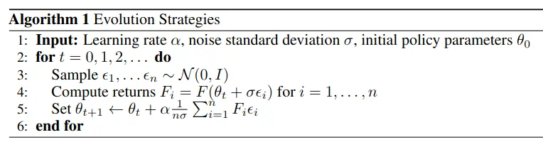
Evolution Strategies

NES

This paper uses NES, where an objective function $F$ acting on parameters $\theta$ is optimized. What makes it a natural evolution strategy is that we are not directly optimizing $\theta$, but optimizing a distribution over parameters (“populations”) $p_{\psi }(\theta )$–itself parametrized by $\psi$– and proceed to maximize the average objective value ${\mathbb{E}}_{\theta \sim p_{\psi }}F(\theta )$ over the population by searching for $\psi$ with stochastic gradient ascent, using the score function estimator for ${\nabla }_{\psi }{\mathbb{E}}_{\theta \sim p_{\psi }}F(\theta )$ similar to REINFORCE.
So gradient steps are taken on $\psi$ like this:

$$\begin{array}{r}{\nabla }_{\psi }{\mathbb{E}}_{\theta \sim p_{\psi }}F(\theta )={\mathbb{E}}_{\theta \sim p_{\psi }}\{F(\theta )\nabla \log p_{\psi }(\theta )\}\end{array}$$

We estimate the gradient by sampling the distribution because we can’t integrate over all possible values of $\theta$.
Their population distribution $p_{\psi }$ is a factored gaussian, the resulting gradient estimator is known as “simultaneous perturbation stochastic approximation”, “parameter-exploring policy gradients”, and “zero-order gradient estimation” (zero order optimization).
The initial population distribution is an isotropic multivariate gaussian, with mean $\psi$ and fixed covariance ${\sigma }^{2}I$.
Initially, we optimize $\psi$ which controls a population distribution $p_{\psi }(\theta )$ that generates parameters $\theta$. However, by fixing $p_{\psi }$ as a Gaussian with mean $\theta$ and variance ${\sigma }^{2}I$, we can simplify this to directly optimizing $\theta$ by simply adding Gaussian noise $ϵ\sim N(0,I)$ during sampling. This transforms the problem from optimizing population distribution parameters ($\psi$) to directly optimizing the mean ($\theta$) of a fixed-form Gaussian, while maintaining exploration through noise injection. The resulting simplified gradient estimator:

$$\begin{array}{r}{\nabla }_{\theta }{\mathbb{E}}_{ϵ\sim N(0,I)}F(\theta +\sigma ϵ)=\frac{1}{\sigma }{\mathbb{E}}_{ϵ\sim N(0,I)}\{F(\theta +\sigma ϵ)ϵ\}\end{array}$$

This noise / gaussian blurring also allows us to train on non-differential / unsmooth environments.

Link to original

Natural Evolution Strategies (NES)

Evolution strategies that use natural gradient descent to update search distribution parameters.
NES optimizes a probability distribution $p_{\psi }(\theta )$ over parameters by maximizing expected fitness:

$$\underset{\psi }{\max }{\mathbb{E}}_{\theta \sim p_{\psi }}[F(\theta )]$$

Updates use the natural gradient ${\tilde{\nabla }}_{\psi }=F^{-1}{\nabla }_{\psi }$ where $F$ is the fisher information matrix.

This ensures the algorithm takes consistent steps in distribution space rather than parameter space - a small parameter change that drastically alters the distribution is scaled appropriately.

Link to original

Financial Computations

Black-Scholes

…

Continue section 3 onwards after ALIFE, finishing probability rabbit hole, and maybe also after optimization bootcamp is out…

’+ https://andrewcharlesjones.github.io/journal/log-derivative.htm

Footnotes

1. We will make one restriction in this review, and that is to problems where the measure $p$ is a probability distribution that is continuous in its domain and differentiable with respect to its distributional parameters.

   ↩

2. Check out this epic visualization of how $f$ and $p_{\theta }$ convolve, and how the sensitivity guides the parameter optimization. ↩

3. Sensitivity here just means the gradient of an expectation, i.e. a measure of how much the expected value changes in response to small changes in parameters. Not really connected to the numerous other uses of the word sensitivity in other contexts, beyond the general idea of responsiveness to change. ↩

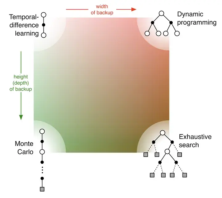
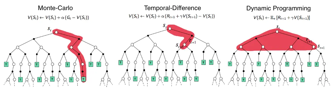
Link to original

monte carlo methods vs temporal difference learning vs dynamic programming

The picture shows the value propagation (“backup”) of a single update step with these three methods:

MC methods require complete episodes to learn, using actual returns $G_t$ to update value estimates. They’re unbiased (as long as there is exploration) but have high variance and require complete episodes (and thus more samples to achieve an accurate estimate, so bad for expensive environments), though truncated returns can also work.

TD bootstraps from existing value estimates after single steps, combining actual rewards with predicted future values. This introduces bias but reduces variance and enables online learning.

DP methods use the full model of the environment to consider all possible next states simultaneously, computing expected values directly. This is most sample-efficient (you don’t need to sample in order to approximate values – at the cost of exhaustive search) but requires a complete model of the environment, and are impractical for large state spaces, even with a perfect model (curse of dimensionality).

MC (left) vs TD

Link to original

https://lilianweng.github.io/posts/2018-02-19-rl-overview/#monte-carlo-methods