Mastering Atari, Go, Chess and Shogi by Planning with a Learned Model

year: 2019
paper: https://arxiv.org/pdf/1911.08265.pdf
website: https://www.deepmind.com/blog/muzero-mastering-go-chess-shogi-and-atari-without-rules
code: PwC Github-GeneralMuZero
connections: Deepmind, reinforcement learning, model-based, Julian Schrittwieser

---

30min Schrittwieser
Schrittwieser blog
Lesswrong blog

Introduction

MuZero is a model-based reinforcement learning algorithm. It builds upon AlphaZero’s search and search-based policy iteration algorithms, but incorporates a learned model into the training procedure.

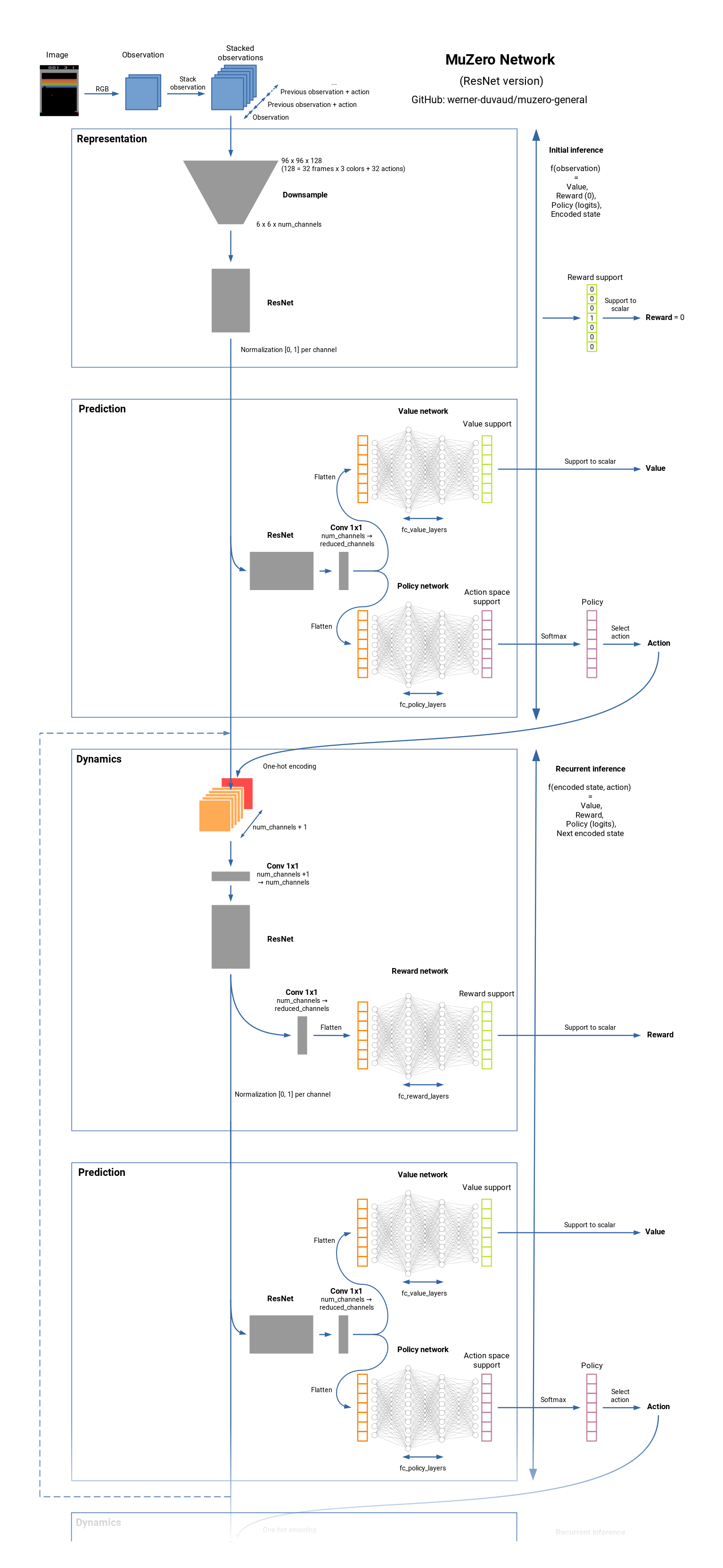
The main idea of the algorithm is to predict those aspects of the future that are directly relevant for planning. The model receives the observation (e.g. an image of the Go board or the Atari screen) as an input and transforms it into a hidden state. The hidden state is then updated iteratively by a recurrent process that receives the previous hidden state and a hypothetical next action. At every one of these steps the model predicts the policy (e.g. the move to play), value function (e.g. the predicted winner), and immediate reward (e.g. the points scored by playing a move). The model is trained end-to-end, with the sole objective of accurately estimating these three important quantities, so as to match the improved estimates of policy and value generated by search as well as the observed reward.

There is no direct constraint or requirement for the hidden state to capture all information necessary to reconstruct the original observation, drastically reducing the amount of information the model has to maintain and predict; nor is there any requirement for the hidden state to match the unknown, true state of the environment; nor any other constraints on the semantics of state. Instead, the hidden states are free to represent state in whatever way is relevant to predicting current and future values and policies. Intuitively, the agent can invent, internally, the rules or dynamics that lead to most accurate planning. ¹

$t\dots$ time
$\theta \dots$ neural net parameters
$o\dots$ observations
$h_{\theta }\dots$ representation net: $h_{\theta }(o_t,o_{t-1},\dots )\mapsto s_k$

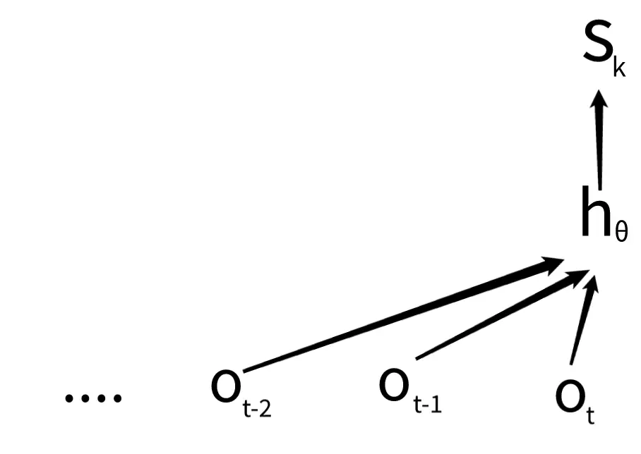
$k\dots$ internal representation timestep
$g_{\theta }\dots$ dynamics net: $g_{\theta }(s_k,a_k)\mapsto s_{k+1},r_{k+1}$

you can use the dynamics net to predict different action trajectories (then the grafik above would look like a tree).
$s_k$ needs to have enough information to predict the reward and the next hidden representation, however, the net is not trained to predict the next observations.

$V_{\pi }(s_k)\dots$ state value funciton
${\pi }_{s_k}\dots$ policy
$f_{\theta }\dots$ prediction net: $f_{\theta }(s_k)\mapsto V(s_k),{\pi }_{s_k}$

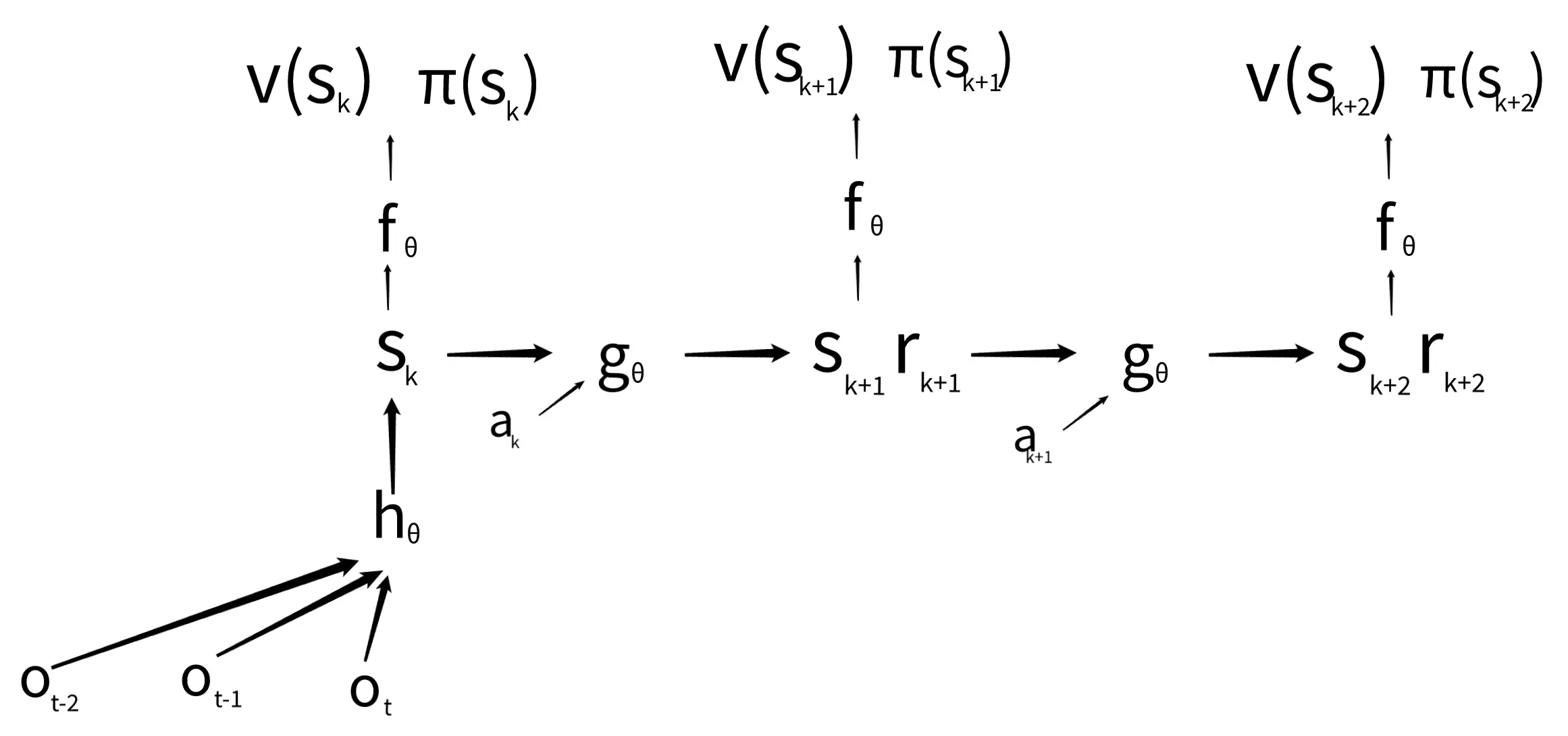
The prediction net can be executed for any state whose value function and distribution over actions ($\pi$) you’re interested in. With a perfectly trained network, we could either use $\pi$ or $V$ to perform the perfect action in any situation.

So in the end the network outputs / models:

• reward: how good was the last action?
• value function: how good is the current position?
• policy: which action is the best to take?

These outputs of the network alone might not be consistent however, if the network is imperfectly trained.
E.g. the network produced a state $s_k$, the policy gives an even distribution over two actions available: left and right. The dynamics function however predicts that if you go left, you’ll get 100 reward forever after and -100 forever after, if you go right. The policy at state $s_k$ is inconsistent with the predicted reward at the next state.

At the very highest level of abstraction, Monte Carlo Tree Search as used by MuZero just uses the neural network to produce policy and state value estimates that are more internally consistent.

“ MCTS” in muzero neither does random simulation nor does it rollout till the end.

The search at each step looks like this:

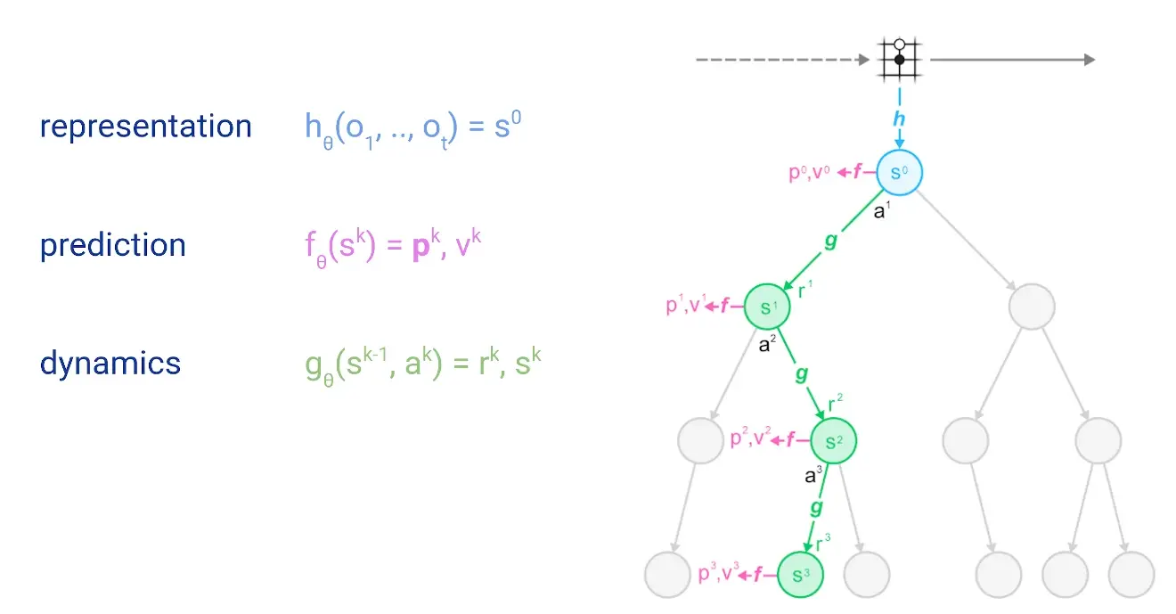
(the grid thingy is supposed to represent a Go board)

On a high level, the model uses these three expereiences to learn:

• observations &
• rewards from the environment
• mcts results over best action

We have $h$ produce $s_{k+n}$ hidden states using actions that the agent took at the corresponding time-steps.
We can train the reward function (dynamics net) by simply checking if it matches the actual environment reward at $s_{t+n}$.

The value function, defined as the expected return of a state given a policy $V(s_t)=E[R|s_t,\pi ]$, could in the simplest case be obtained by just letting the policy gather lots of playouts from the state using the policy and average the sum of future rewards from the environment, which will definitionally converge towards the state-value function for that state and policy.
Since this is a bit slow, we improve the performance by bootstrapping:
Instead of calculating, as described above: $V(s_t)=E[r_{t+1}+r_{t+1}+\dots r_{t+N}|s_t,\pi ]$,
we set the target for the value function as: $V(s_t)\to r_{t+1}+r_{t+2}+r_{t+3}+V(s_{t+4})$
So we move $V$ towards the value on the right, consisting of actual rewards + estimate of the state-value of a future state. This way we don’t have to collect actual rewards all the way through but $V$ still converges to the right value by encorporating experienced rewards.

The target for the policy net is the improved / more consistent policy distribution generated for each state by MCTS.

1. random network learns to predict rewards it ecounters
2. rewards shape the value function
3. mcts driven by learnt rewards and value function improves policy (action selection)
4. value function targets shift because the policy changed
5. MCTS also can explore more deeply with better policy
6. Even already trained on data can become relevant again, as it will now look at it with a new policy ²

The “chain of improvement” could be sketeched as: $V,r\to \text{MCTS}\to \pi \to \text{MCTS}$

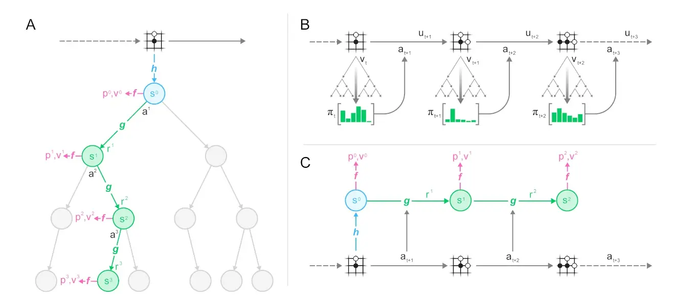
To explain the above image: We start of in a state $s_0$, do MCTS (A), with the collected stats choose an action (B, episode generation), $g$ predicts the dynamics, $f$ gives us new functions for doing another MCTS for the next step (C, training).

MuZero’s “MCTS” in detail

First, we simulate:
As seen above, we start with the first hidden state representaiton $s_0$ as the root node. Then at each node (state $s$), we use the scoring function $U(s,a)$ ($U$ for upper confidence bound), to compare different actions and choose the most promising one. MuZero’s scoring function combines a “prior estimate” ³ $p(s,a)$ with the value estimate for $v(s,a)$:

$$\begin{array}{r}U(s,a)=\underset{\text{exploitation}}{\underbrace{v(s,a)}}+c\cdot \underset{\text{exploration}}{\underbrace{p(s,a)}}\end{array}$$

So the value for each next node is determined by the raw policy prediciton and the state prediction (doesn’t need to be scaled itself, should be in $[0,1]$ just like the prior).
$c$ is a scaling factor to ensure that the influence of the prior diminishes (resets with every mcts) as we gather more simulations and $v$ becomes more accurate, balancing exploration and exploitation.
In MuZero,

$$\begin{array}{r}c=\frac{\sqrt{{\sum }_{b}n(s,b)}}{1+n(s,a)}\cdot \left(c_1+\log \left(\frac{{\sum }_{b}n(s,b)+c_2+1}{c_2}\right)\right)\end{array}$$

where $n(s,a)$ are the number of visits for action $a$ from state $s$, and $c_1=1.25$ and $c_2=19652$ ⁴ are constants to influence the importance of the prior relative to the value estimate. In the beginning, where $c_2\gg n$, the $\log$ term becomes $0$. In this case, the formula simplifies to $c_1\cdot \frac{\sqrt{{\sum }_{b}n(s,b)}}{1+n(s,a)}$. ⁵

So each time an action is selected (via $U$), we increase $n(s,a)$, putting more emphasis on what we learn from our monte carlo exploration as opposed to what we initially guessed with our policy. The evaluation results ($p$ and $v$) get stored into the node. Simulation continues until we reach a leaf that has not yet been expanded.

$$a^k=\left\{\arg \underset{a}{\max }Q(s,a)+P(s,a)\frac{\sqrt{{\sum }_{b}N(s,b)}}{1+N(s,a)}\left(c_1+\log \left(\frac{{\sum }_{b}N(s,b)+c_2+1}{c_2}\right)\right)\right\}$$

$Q(s,a)\dots$ average $Q\text{-value}$ after simulations (of all the sub-branches of one of a root node).

Expansion: Once a node has reached a certain number of evaluations, it is marked as “expanded”. Being expanded means that children can be added to a node; this allows the search to proceed deeper. In MuZero, the expansion threshold is $1$, i.e. every node is expanded immediately after it is evaluated for the first time. Higher expansion thresholds can be useful to collect more reliable statistic before searching deeper but is generally not useful when using a deterministic evaluation function (like standard neural nets, as the explored path would always be the same), but most useful with stochastic evalution functions, like with classic mcts, where you use random rollouts.
TLDR: You need to visit all

Backpropagation: Finally, the value estimate from the neural network evaluation is propagated back up the search tree; each node keeps a running mean of all value estimates below it. This averaging process is what allows the UCB formula to make increasingly accurate decisions over time, and so ensures that the MCTS will eventually converge to the best move.

Intermediate Rewards

In envs with intermediate rewards, we just modify the UCB formula a bit:

$$\begin{array}{r}U(s,a)=r(s,a)+\gamma \cdot v(s^{\prime })+c\cdot p(s,a)\end{array}$$

where $r(s,a)$ is the reward observed in transitioning from state $s$ by choosing action $a$, and $\gamma$ is the classic discount factor that describes how much we care about the future rewards.

Reward scaling

As hinted above, rewards can have arbitrary scale, we need to normalize the combined reward/value estimate to lie in the interval $[0,1]$ before combining it with the prior:

$$\begin{array}{r}U(s,a)=\frac{r(s,a)+\gamma \cdot v(s^{\prime })-q_{\min }}{q_{\max }-q_{\min }}+c\cdot p(s,a)\end{array}$$

where $q_{\min }$ and $q_{\max }$ are the minimum and maximum $r(s,a)+\gamma \cdot v(s’)$

Episode Generation

On a high level, the flow for repeatedly applying mcts is:

• Run a search in the current state $s_t$​ of the environment.
• Select an action $a_{t+1}$ according to the statistics ${\pi }_t$​ of the search.
• Apply the action to the environment to advance to the next state $s_{t+1}$​ and observe reward $u_{t+1}$
• Repeat until the environment terminates.

Action selection can either be greedy - select the action with the most visits - or exploratory: sample action $a$ proportional to its visit count $n(s,a)$, potentially after applying some temperature $t$ to control the degree of exploration:

$$\begin{array}{r}p(a)={\left(\frac{n(s,a)}{{\sum }_{b}n(s,n)}\right)}^{1/t}\end{array}$$

For $t\to 0$, we recover greedy action selection; $t=\infty$ is equivalent to sampling actions uniformly.

Losses

(notation from Efficient Zero paper)

$$\mathcal{L}(u_t,r_t)+{\lambda }_1\mathcal{L}({\pi }_t,p_t)+{\lambda }_2\mathcal{L}(z_t,v_t)$$

The training losses for the three quantities estimated by MuZero are:

• reward: cross-entropy between reward from the environment $u_t$ and the reward from the prediction of the dynamics net, $r_t=\mathcal{R}(s_t,a_t)$
• policy: cross-entropy between MCTS visit count distribution ${\pi }_t$ and the predicted policy “policy logits” from $p_t=\mathcal{P}(s_t)$
• value: cross-entropy or MSE between discounted sum of N rewards with bootstrapping $z_t={\sum }_{i=0}^{k-1}{\gamma }^i{u}_{t+1}$⁶, where $u$ is the reward from the replay buffer, and the stored search value or target network estimate and value from the prediction function.

MuZero does not explicitly learn the environment model. Instead, it solely relies on the reward, value, and policy prediction to learn the model.

Reanalyse

Basically, you save a past trajactories in a reanalyse buffer, because you can learn new things from them once your network has improved.

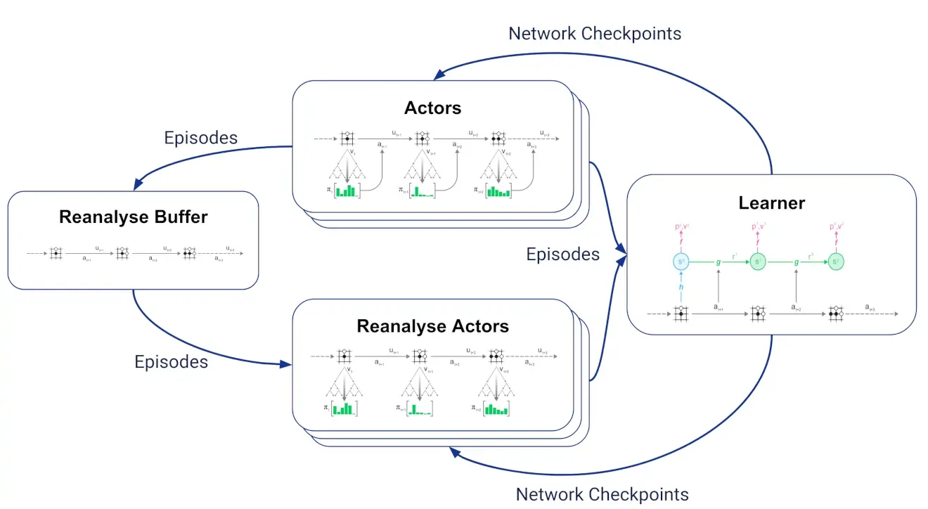
In our implementation of MuZero, there is no separate set of actors for reanalyse: We have a single set of actors which decide at the start of each episode whether to start a fresh trajectory interacting with the environment or to reanalyse a stored trajectory. - Schrittwieser

Related

implicit world models
reinforcement learning

Appendix

Gobbled together implementation details…

Performance consideration and simulation ballpark: (~2022)

If you want to run a large number of small searches in parallel (say 50 simulations per move and 64 games at the same time), then JAX can be feasible. If you only want to run a single very large search (say Go or some abstract planning problem), then you’ll get better performance with C++ or Rust.

Virtual loss through paralellization … decreases some potential bad effect in mcts.

It seems that if the very first child of the root node has a somewhat higher prior probability than the rest of root’s children, it may take a lot of simulation iterations to expand some other child of the root (if we assume that the first child has a normalized value somewhat above zero, which it might).Here, assuming that the first child’s normalized value keeps around 0.4, we will spend 14 simulations until we consider any other action. If our simulation budget is limited to, say, 25 iterations, this node will get at least 14/25=0.56 of all visits, which is actually higher than the prior probability we’ve started with, even if other children are better! Can’t this lead to asymmetries in prior distribution reinforcing themselves and policy eventually collapsing?
Also a somewhat related question. Given that during training we only unroll our dynamics model for 5 steps, would it make sense to go deep into some branches during simulation? We should probably quickly get into an area of the latent space where our value and policy predictions are complete garbage, thus ruining value estimates for the nodes higher above. It feels like maximum simulation depth should be limited for MuZero to work, but I haven’t seen any mentions of that in the paper.
→ Schrittwieser answer:
I think you are right about this effect. I think the reason why we often notice it less is a side effect of parallelizing the search using virtual loss: up to N evaluations are started in parallel, add a temporary K extra visits until the evaluation has arrived (decreasing the averaged value, thus virtual loss). For Atari we use N=4, K=10.
Another option is presented by our recent paper, Policy improvement by planning with Gumbel I’ll write a post about this one soon.

Terminal states policy loss & labels

Another question that came up: how exactly are terminal states handled during training?
During selfplay they’re not handled at all, MCTS just continues searching past them as if nothing has happened, and then when a terminal state is actually reached in the environment the game is stopped.
But during training, what if the K=5 unrolling gets us past a terminal state? There is this paragraph in the methods section of the paper:

Inside the tree, the search can proceed past a state that would terminate the simulator. In this case, the network is expected to always predict the same value, which may be achieved by modelling terminal states as absorbing states during training.
And the pseudocode has this:
# States past the end of games are treated as absorbing states. targets.append((0, last_reward, []))

Which is not constant value, but constant reward. Which of these is right? Is it different for board games vs domains with nonzero reward?
Additionally the policy output is empty, does this mean the prediction network f is expected to predict that there are no available moves any more by predicting an all-zero policy? How does this work with the softmax at the end of the network? Or is there simply no policy loss for post-terminal states?
→Schrittwieser answer:
There is no policy loss for post-terminal states, we handle this by masking the loss if the policy label is all 0.
If predicting a reward, then post-terminal states have constant 0 labels for both value and reward. If predicting only value, no reward (as in board games or other environments that only have a single terminal reward) then post-terminal states have a constant value label.

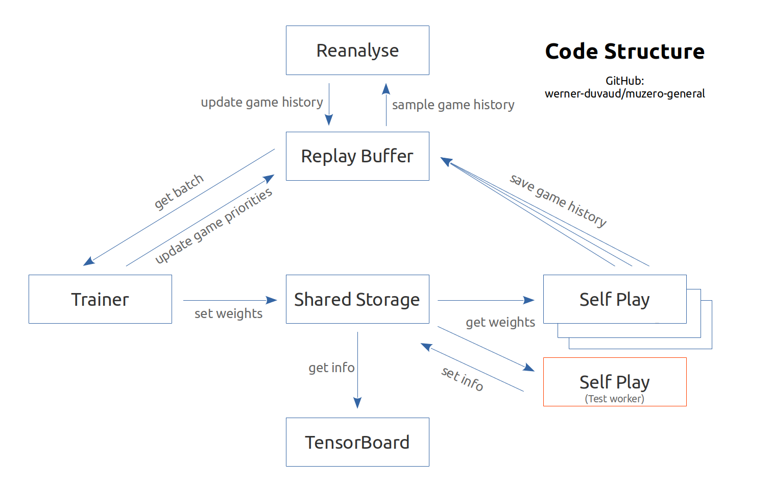
Diagrams

Footnotes

1. https://paperswithcode.com/method/muzero ↩

2.  For example, in tests on the Atari suite, this variant - known as MuZero Reanalyze - used the learned model 90% of the time to re-plan what should have been done in past episodes. ↩

3. “prior estimate” in this case means an estimate before taking information from mcts into account. ↩

4. The idea behind c_2 is to ensure that the prior still has some influence at very high simulation counts, e.g. when searching for hundreds of thousands or millions of simulations per move in Go. The exact value for it doesn’t matter much, only the order of magnitude.

   ↩

5. ${\sum }_b(s,b)\dots$ total number of visits a node has (summing over all the actions). ↩

6. For board games, the discount $\gamma$ is $1$ and the number of TD steps infinite finite, so this is just prediction of the Monte Carlo return (winner of the game). ↩