transformer

---

TOC:

• High level facsts
• Components

High level facsts

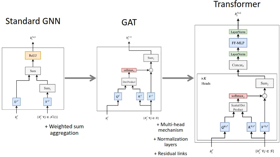
The transformer is actually a graph neural network processor.

(… pretty much everything is nowadays)
The native representation that the transformer operates on is sets that are connected by edges, in a directed way.
This frees neural net computation form the burden of euclidian space.
Previously you had to conform your compute to a 3D layout, in attention it’s just sets. See also: ^c1f58f.
This message-passing architecture (see ^159181 for an explanation) is general (complete) and powerful (efficient), able to cover many real-world algorithms in a small number of compute steps.

Limitation: Can’t draft / edit.

The autoregressive sampling - sampling a token and then commiting to it - that is used in decoder-only transformers is one of the biggest weaknesses.
Maybe we might find hybrids with diffusion or some other way to incorporate editing into the autoregressive process.

The transformer is super flexibly: Information can easily be plugged in.

Just chop the data into pieces, add it into the mix, self-attend over everything.
Even if it doesn’t make much sense / has zero inductive bias or whatsoever, e.g. with ViT or whisper (any audiotransfomer, e.g. “Conformer”), where you literally just chop up images or audio spectrograms and feed them into the transformer. Or the decision transformer, where you put states, actions, rewards into the transformer, pretend it is language and model the sequence of that.

The transformer is like a computer optimizable by gradient descent.

Transclude of Language-Models-are-Few-Shot-Learners#^260d49

The shallow architecture of the transformer allows it to run very efficiently on GPUs.

This is in contrast to RNNs, which have a very long, thin compute graph. Apart from paralellization, this also complicates the flow of gradients, where it’s better to have fewer steps.

Transclude of inductive-bias#^a88119

Transformer == GNN with extra steps

Source 1 2

Transformers and The Bitter Lesson (from The Bittersweet Lesson)

→ If it’s possible for a human domain expert to discover from the data the basis of a useful inductive bias, it should be obvious for your model to learn about it too, so no need for an inductive bias.
→ Instead focus on building biases that improve either scale, learning or search .
→ In the case of sequence models, any bias towards short-term dependency is needless, and may inhibit learning (about long-term dependency).
→ Skip connections are good because they promote learning.
→ MHSA is good because it enables the Transformer to (learn to) perform an online, feed-forward, parallel ‘search’ over possible interpretations of a sequence.

Inner workings / Components

Task

The transformer accepts a set of observations $\mathbb{X}=\{{\mathbf{x}}_1,{\mathbf{x}}_2,\dots ,{\mathbf{x}}_T\}$, (${\mathbf{x}}_t$ could be a word embedding, image patch, …), and aims to predict missing elements of that set (usually).
The missing elements could be in the future, i.e $x_{t>T}$ (e.g. in autoregressive language modelling), or could be a missing part of a sentence or image, i.e. $\{{\mathbf{x}}_1=\text{the},{\mathbf{x}}_2=\text{cat},{\mathbf{x}}_3=\text{sat},{\mathbf{x}}_4=\text{?},{\mathbf{x}}_5=\text{the},{\mathbf{x}}_6=\text{mat}\}$.

At the core of the transformer is the self-attention mechanism, which often is augmented by using multiple heads: multi-head attention.
Before feeding into self-attention, we often project input to a lower dimension (dimensionality reduction) e.g. using learned embeddings.
The transformer learns the patterns in this embedding space (where similar are grouped together → similar vectors will be treated similarly).
Padding tokens are added so that the input retains a constant shape of the maximum sequence length.

finish refactor

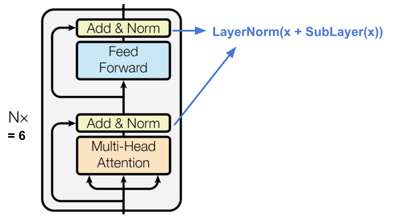
The output from self-attention $\mathbf{Y}$ is then passed through a deep network $f_{\theta }$, typically consisting of residual connections and layer normalization (nowadays PreNorm). This output $\mathbf{Z}=f_{\theta }(\mathbf{Y})$ can then be used for prediction, or
sent through subsequent transformer blocks.
At the end of the transformer blocks in the original paper, they put a “de-embedding” matrix, the same shape as the embedding matrix, but with the number of rows and columns flipped, on which softmax is applied to get probabilities for the next token:

Encoder

• A stack of $N=6$ identical layers. (in the original paper)
• Each layer has a multi-head attention layer and a simple position-wise fully connected feed-forward network (linear).
  • Each head 64 dimensional (as standard)
• The MLP adds extra complexity / ability for post-process new information and prepare for next block.
  • usually inner dimensionality of MLP is 2-8 x larger than $d_{model}$ (dimensionality of original input $x$), 4x in paper.
  • wider layer → faster, parallelizable execution.
• After* both, layer normalization is applied. (Faster training, small regularization, features of simmilar magnitude among elements in a sequence)
  • No BatchNorm, esp. because small batches in Transformers (require lot of GPU RAM)
  • BatchNorm performs particularly bad in language: Many very rare words which are important for a good distribution estimate → high variance
  • • Applied after MHA and FFN in original paper, but directly on the inputs before going into them is more common now, see summary below (src: Karpathy explains).
• Lastly, both adopt a residual connection
  • Crucial for smooth gradient flow through the model (some models contain more than 24 stacked blocks)
  • Without it, positinal information would be lost (MHA ignores position).

All the sub-layers ($N$) output data of the same dimension.

Overall it calculates (original paper):
$FFN(x)=max(0,x{W}_1+b_1)W_2+b_2$

$$\begin{gathered} \text{displaylines}LayerNorm(x+Multihead(x,x,x)) \\ LayerNorm(x+FFN(x)) \end{gathered}$$

newer version:

$$\begin{gathered} \text{displaylines}x+Multihead(LayerNorm(x,x,x)) \\ x+FFN(LayerNorm(x)) \end{gathered}$$

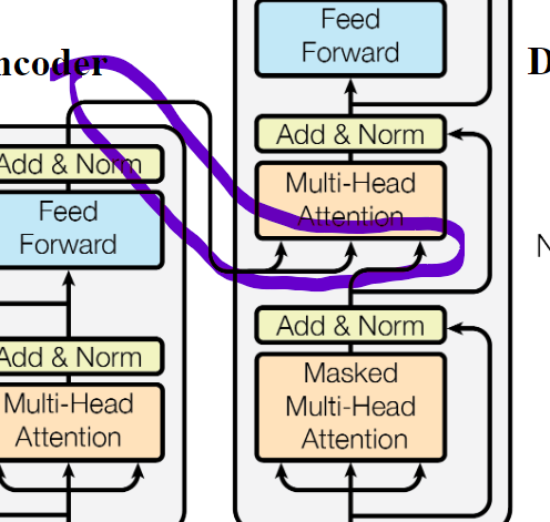
cross-attention - Encoder Decoder Intuition

In the original task of the paper, translation, the encoder gets shown the e.g. french sentence.

It is not masked so all tokens (words) can talk to eachother as much as they want (to “get the meaning of the sentence”).
The keys and values of the encoder are input to the second MHA of the decoder (all $N$ blocks), so essentially, the decoder has the information of the past english tokens and the information of the fully encoded french sentence.

Decoder TODO

positional encodings

Fixed values added to input in order to keep positional information. (Residual connections needed aswell)
Essentially like adding binary counting vectors to the input, but with continous values.

Properties / Limitations

Shape size intuition (TODO … refactor this)

voc … vocabulary size | multiple (tens) of thousands
seqL … sequence length | 2048 in GPT3
d_model … number of hidden dimensions in embedding space throughout model | 512 in Vaswani
(voc x d_model) ← word embedding; positional embedding

Time and space complexity

Memory requirement for transformersscales quadratically with evry Token added, since every Token attends to every other Token, like in a fully meshed topology:

$$\frac{T\cdot (T-1)}{2}\Rightarrow O(T^2)$$

($T$ … Tokens form connections with every other $T$ except itself, division removes duplicates)

	Time	Space
Transformer	$O(T^{2}d)$	$O(T^2+Td)$
RWKV	$O(Td)$	$O(d)$
$d$ … embedding dimension (constant)
(RWKV - Reinventing RNNs for the Transformer Era)

Variations and Sucessors

Improvements

The only fundamental change to the architecture throughout the years has been swapping the order of the layernorm:

Transclude of PreNorm#^ref

Variations

ViT
Transformer with memory (lucidrains)
GPT
Music Transformer: Generating Music with Long-Term Structure Paper

Code

https://github.com/lucidrains/robotic-transformer-pytorch/blob/main/robotic_transformer_pytorch/robotic_transformer_pytorch.py

References

LLM

Best one:
→ Stanford CS25: V2 I Introduction to Transformers w/ Andrej Karpathy ←

Super good first intuition (and walkthrough all components) Assembly AI Transformers for beginners
In-depth tensorflow article / colab
Goated Karpathy GPT walkthrough .
Illustrated Transformer
CodeEmporium entire encoder ; Self-Attention with nice experimenting code; … | Video: Tutorial(uses einops)
Annotated Transformer (With Attention visualization, full code)
Youtube: Sentence Tokenization in Transformer Code from scratch - Code Emporium
Theory from scratch (e2eml) (a bit dry and long and not practical)
Relating transformers to models and neural representations of the hippocampal formation