Transformer Squared - Self-Adaptive LLMs

year: 2025/01
paper: https://arxiv.org/pdf/2501.06252
website: https://sakana.ai/transformer-squared/ | https://x.com/SakanaAILabs/status/1879325924887613931
code: https://github.com/SakanaAI/self-adaptive-llms
connections: sakana AI, transformer, SVD

---

Vibe check: Cool, but overhyped and has been done before.

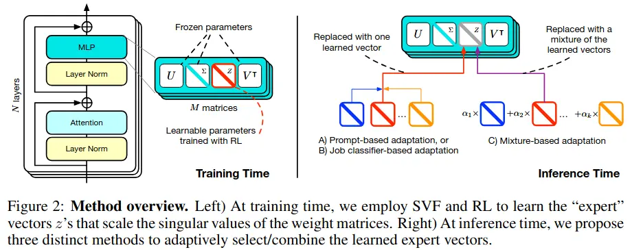
This paper introduces a parameter efficient finetuning technique by scaling the singular values of the weight matrices. The motivation is that pretrained weights already contain vast abstract knowledge necessary for most tasks, and the fine-tuning process should only emphasize / make certain features or capabilities more expressible.

They decompose the weight matrix into $W=U\Sigma V^T$ → $y={\sum }_{i=1}^r{\sigma }_i{u}_i{v}_i^{T}x$, where each $u_i{v}_i^T$ independently processes the input, providing an orthogonal contribution to the layer’s outputs, with the singular value ${\sigma }_i$ modulating the degree of the contribution.

$U,\Sigma ,V$ are all frozen parameters from a pretrained model. $\Sigma$ gets scaled via element-wise multiplication by a learnt adaptation vector $z\in {\mathbb{R}}^r$, giving us new weight matrices $W^{\prime }=U{\Sigma }^{\prime }{V}^T$, where ${\Sigma }^{\prime }=\Sigma \otimes \text{diag}(z)$.

Key benefits:

• Tiny amount of parameters to adapt
• Preserves original information
• High composability → interpretable; distinct/explicit experts
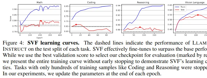
• Regularized fine-tuning: Only modifying the magnitude of pre-existing singular components allows to fine-tune without risking overfitting, severe collapse and with only “hundreds of datapoints”.

They simply use REINFORCE, with rewards $r\in \{-1,1\}$ based on correctness of answer $y_i$ for a prompt $x_i\in D$ and add a KL-penality to the loss to prevent the fine-tuned policy diverging from the original one. ¹
The final objective function is

$$J({\theta }_z)=\mathbb{E}[\log ({\pi }_{{\theta }_{W^{\prime }}})({\hat{y}}_i\mid x_i)r({\hat{y}}_i,y_i)]-\lambda D_{\text{KL}}({\pi }_{{\theta }_{W^{\prime }}}\parallel {\pi }_{{\theta }_W})$$

where ${\pi }_{{\theta }_{W^{\prime }}}$ is the policy of the fine-tuned model with weight matrices $W^{\prime }$, ${\pi }_{{\theta }_W}$ the policy of the original model, and $\lambda$ the KL-penality coefficient.

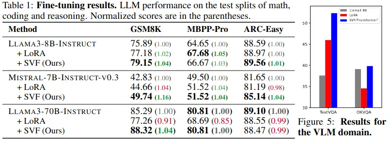
Fine-tuning with RL works well with SVF, less well with LoRa / other methods, which are fine-tuned with next-token prediction.

In the training phase, they “manually” train separate expert vectors for each capability/domain out of a fixed set (math, coding, reasoning, other), by fine-tuning on domain-specific datasets.
Optionally, depending on the inference method, they train a classification expert vector $z^c$ using examples from all domains to help with task identification.

During inference, they employ a two-pass mechanism to choose the experts
First Pass: Identify the task type and determine which expert(s) to use, via one of these strategies:

• Prompt-based: Runs the base model with a classification prompt to categorize the task
• Classification Expert: Uses a pre-trained classification expert $z^c$ to identify the task
• Few-shot: Evaluates different combinations (linear interpolations) of experts on held-out examples using coefficients learnt by CEM. ²

Second Pass: Actually solve the task using the adapted weights. Uses the identified expert vector(s) to modify the model’s weights via SVF:

• Single expert case: Directly uses the identified expert’s $z$ vector
• Few-shot case: Uses the learned mixture $z^{\prime }={\sum }_{k=1}^K({\alpha }_k{z}_k)$ where $a_k$ are CEM-optimized coefficients

While this requires two forward passes, the paper shows the first pass is typically much faster since it doesn’t need to generate long outputs - for example, in their experiments on ARC-Challenge, the first pass only takes about 47% of the time of the second pass, while for longer-form tasks like MATH, it takes only about 13%.

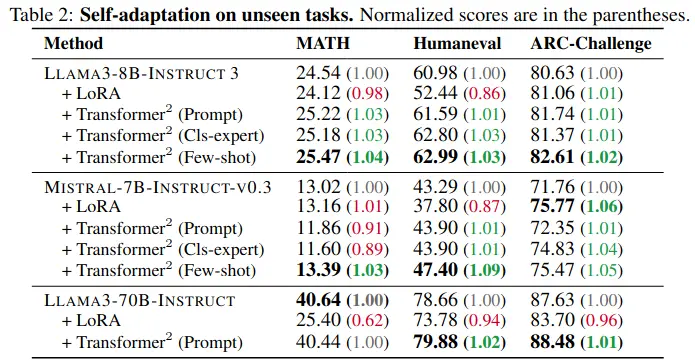
Results show that few-shot adaptation generally performs best. Generally it’s a few percentage points better than LoRa (but altogether much better than the base).
Transformer² improves performance on unseen tasks too, by a few percentage points, whereas LoRa sometimes even degrades (same with the prompt and cls-expert based inference methods, they are better, but less consistently better, esp. on math).

Interestingly, they also show that experts trained on pure language tasks can help with vision-language tasks, suggesting the adaptations capture general capabilities rather than just domain-specific knowledge.

Some experiment details

For a given pre-trained model, they first train multiple SVF experts, one for each core capability/domain:

Task Selection: They choose datasets representing distinct capabilities:

• GSM8K for mathematical reasoning
• MBPP-pro for coding
• ARC-Easy for general reasoning

Expert Training: For each task, they train a separate expert vector z using SVF and REINFORCE:

• Split the dataset into equal training and validation parts
• Use AdamW optimizer with learning rate 2×10⁻³ and cosine decay
• Apply gradient clipping and early stopping
• Select best KL penalty coefficient λ based on validation performance

Layer Coverage: For most models (except LLAMA3-70B and vision tasks), they train experts for all layers. For the larger models, they only adapt half the layers to reduce memory usage while maintaining significant performance improvements.

“During the training of LLAMA3-8B-INSTRUCT on the vision language tasks, we apply a small negative reward (-0.1) for training stability.”

def cem_step(mu, sigma, num_elites, num_samples):
	samples = np.random.normal(loc=mean, scale=sigma, size=num_samples)
	scores = evaluate(samples)
	elites = samples[np.argsort(scores)[-num_elites:]]
	new_mu = np.mean(elites, axis=0)
	new_sigma = np.std(elites, axis=0)
	return (new_mu, new_sigma)

Footnotes

1. See ^1d3dce for the theoretical motivation behind this. Though penality used here does not compare the policy from the previous step to the current policy, but the current policy to the one before fine-tuning. ↩

2. CEM iteratively samples different combinations of coefficients, evaluates performance on the few-shot examples, and updates the sampling distribution toward better-performing combinations. ↩